Final map

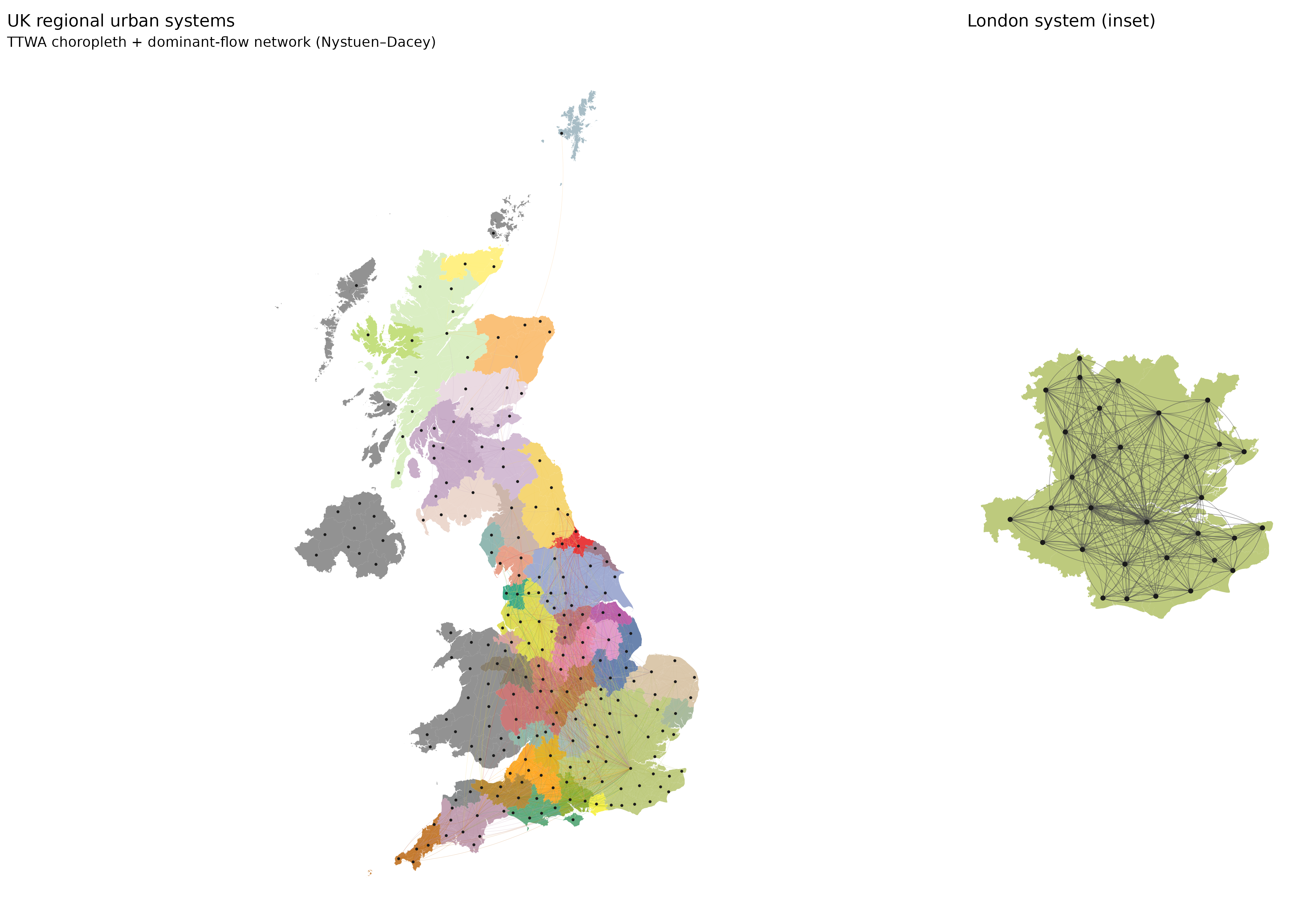
This chapter produces the publication-style cartogram: choropleth TTWA fill by regional system, curved edges weighted by flow, an extended regional colour palette (42+ systems after full UK coverage), a London inset composed with patchwork, and an interactive Leaflet version below the static figure.

Previous: Partition
Next: Project overview

suppressPackageStartupMessages({
  library(sf)
  library(ggraph)
  library(ggplot2)
  library(patchwork)
  library(scales)
  library(tidyverse)
  library(tidygraph)
  library(tidyverse)
  library(here)
})

proj_dir <- here::here("projects", "uk-urban-systems-network")
data_dir <- file.path(proj_dir, "data")
fig_dir <- file.path(proj_dir, "figures")
dir.create(data_dir, recursive = TRUE, showWarnings = FALSE)
dir.create(fig_dir, recursive = TRUE, showWarnings = FALSE)

ttwa_boundaries <- readRDS(file.path(data_dir, "ttwa_boundaries.rds"))
od_ttwa_pairs <- readRDS(file.path(data_dir, "od_ttwa_pairs.rds"))
ttwa_centroids <- readRDS(file.path(data_dir, "ttwa_centroids.rds"))
partition_labels <- readRDS(file.path(data_dir, "partition_labels.rds"))

# London 2011 TTWA (name match), not the largest regional system by member count
LONDON_ANCHOR <- ttwa_boundaries |>
  st_drop_geometry() |>
  filter(str_detect(ttwa11nm, regex("London", ignore_case = TRUE))) |>
  pull(ttwa11cd) |>
  first()

message("London TTWA anchor: ", LONDON_ANCHOR)

London TTWA anchor: E30000234

26-colour regional palette

source(file.path(proj_dir, "R", "map_interactive.R"))

n_regions <- n_distinct(partition_labels$region_id)
region_colors <- region_palette(n_regions)
message("Regional systems: ", n_regions)

Regional systems: 41

Main cartogram

ttwa_regions <- ttwa_boundaries |>
  left_join(partition_labels, by = "ttwa11cd")

edges_for_plot <- od_ttwa_pairs |>
  left_join(partition_labels |> rename(from = ttwa11cd), by = c("origin_ttwa" = "from"))

node_xy <- ttwa_centroids |>
  transmute(
    ttwa11cd,
    x = sf::st_coordinates(geometry)[, 1],
    y = sf::st_coordinates(geometry)[, 2]
  )

edge_segments <- edges_for_plot |>
  left_join(node_xy |> rename(origin_ttwa = ttwa11cd, x = x, y = y), by = "origin_ttwa") |>
  left_join(node_xy |> rename(dest_ttwa = ttwa11cd, xend = x, yend = y), by = "dest_ttwa")

p_main <- ggplot() +
  geom_sf(data = ttwa_regions, aes(fill = factor(region_id)), colour = NA, alpha = 0.85) +
  geom_curve(
    data = edge_segments,
    aes(x = x, y = y, xend = xend, yend = yend, linewidth = flow, colour = factor(region_id)),
    alpha = 0.35,
    curvature = 0.15,
    inherit.aes = FALSE,
    show.legend = FALSE
  ) +
  geom_point(
    data = node_xy,
    aes(x = x, y = y),
    size = 0.4,
    colour = "grey10",
    inherit.aes = FALSE
  ) +
  scale_fill_manual(values = region_colors, guide = "none") +
  scale_colour_manual(values = region_colors, guide = "none") +
  scale_linewidth_continuous(range = c(0.1, 1.5), guide = "none") +
  coord_sf(crs = sf::st_crs(ttwa_boundaries), default_crs = sf::st_crs(ttwa_boundaries)) +
  labs(
    title = "UK regional urban systems",
    subtitle = "TTWA choropleth + dominant-flow network (Nystuen–Dacey)"
  ) +
  theme_void()

London inset

london_nodes <- partition_labels |>
  filter(anchor_ttwa == LONDON_ANCHOR) |>
  pull(ttwa11cd)

london_sf <- ttwa_regions |> filter(ttwa11cd %in% london_nodes)
london_edges <- edge_segments |>
  filter(origin_ttwa %in% london_nodes, dest_ttwa %in% london_nodes)
london_xy <- node_xy |> filter(ttwa11cd %in% london_nodes)

bb <- sf::st_bbox(london_sf) + c(-0.15, -0.15, 0.15, 0.15)

p_london <- ggplot() +
  geom_sf(data = london_sf, aes(fill = factor(region_id)), colour = NA, alpha = 0.9) +
  geom_curve(
    data = london_edges,
    aes(x = x, y = y, xend = xend, yend = yend, linewidth = flow),
    colour = "grey30",
    alpha = 0.5,
    curvature = 0.2,
    inherit.aes = FALSE
  ) +
  geom_point(data = london_xy, aes(x = x, y = y), size = 1.2, colour = "grey10", inherit.aes = FALSE) +
  scale_fill_manual(values = region_colors, guide = "none") +
  scale_linewidth_continuous(range = c(0.2, 2), guide = "none") +
  coord_sf(
    xlim = c(bb["xmin"], bb["xmax"]),
    ylim = c(bb["ymin"], bb["ymax"]),
    crs = sf::st_crs(ttwa_boundaries),
    default_crs = sf::st_crs(ttwa_boundaries),
    expand = FALSE
  ) +
  labs(title = "London system (inset)") +
  theme_void()

Interactive cartogram

Full-UK Leaflet version of the choropleth and dominant-flow network (edges with flow ≥ 100). Rebuilds _static/uk-urban-systems-network/maps/07_final_map_interactive.html when this cell runs.

suppressPackageStartupMessages({
  library(leaflet)
  library(htmlwidgets)
  library(htmltools)
  library(IRdisplay)
})

source(file.path(proj_dir, "R", "map_interactive.R"))

edge_segments_leaflet <- prepare_edge_segments(od_ttwa_pairs, ttwa_centroids, min_flow = 100L)

map_final <- leaflet_ttwa_network(
  ttwa_boundaries,
  partition_labels,
  edge_segments_leaflet,
  mode = "final"
)

include_leaflet_map(map_final, "UK regional urban systems (interactive)", "07_final_map_interactive")

Input to asJSON(keep_vec_names=TRUE) is a named vector. In a future version of jsonlite, this option will not be supported, and named vectors will be translated into arrays instead of objects. If you want JSON object output, please use a named list instead. See ?toJSON.

Input to asJSON(keep_vec_names=TRUE) is a named vector. In a future version of jsonlite, this option will not be supported, and named vectors will be translated into arrays instead of objects. If you want JSON object output, please use a named list instead. See ?toJSON.

Input to asJSON(keep_vec_names=TRUE) is a named vector. In a future version of jsonlite, this option will not be supported, and named vectors will be translated into arrays instead of objects. If you want JSON object output, please use a named list instead. See ?toJSON.

Input to asJSON(keep_vec_names=TRUE) is a named vector. In a future version of jsonlite, this option will not be supported, and named vectors will be translated into arrays instead of objects. If you want JSON object output, please use a named list instead. See ?toJSON.

Input to asJSON(keep_vec_names=TRUE) is a named vector. In a future version of jsonlite, this option will not be supported, and named vectors will be translated into arrays instead of objects. If you want JSON object output, please use a named list instead. See ?toJSON.

Input to asJSON(keep_vec_names=TRUE) is a named vector. In a future version of jsonlite, this option will not be supported, and named vectors will be translated into arrays instead of objects. If you want JSON object output, please use a named list instead. See ?toJSON.

Warning message in file(file, ifelse(append, "a", "w")):
“cannot open file '/Users/areeslindley/Documents/Git_repositories/projects-website/.cursor/debug-0556ee.log': No such file or directory”

UK regional urban systems (interactive)

Compose and export

p_final <- p_main + p_london + plot_layout(widths = c(3, 1))

fig_final <- file.path(fig_dir, "07_final_map.png")
ggsave(fig_final, p_final, width = 14, height = 10, dpi = 300)
invisible(fig_final)

Warning message:
“`geom_curve()` is not implemented for non-linear coordinates”

Warning message:
“`geom_curve()` is not implemented for non-linear coordinates”

Data sources

---

Next: Project overview →