Images & Labels

Navigation: ← Previous: Project Overview | Next: Classical Models →

BreastMNIST 128×128 ultrasound: official splits, class balance, and what malignant vs benign looks like at this resolution.

Disclaimer. Educational benchmark only — not a diagnostic tool. Images are centre-cropped/resized BUSI scans at 128×128, far coarser than a clinical workstation.

The task

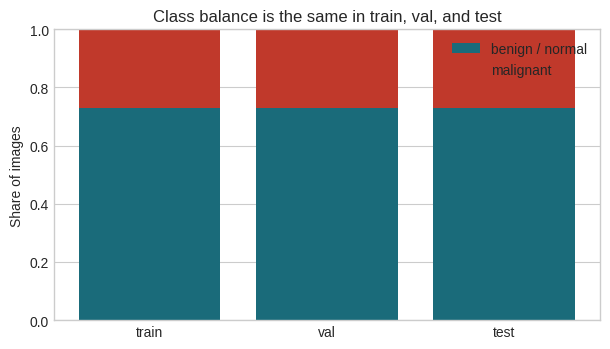
Each image is a breast ultrasound patch labelled malignant or benign/normal. MedMNIST stores malignant as class 0; we remap so that 1 = malignant (the positive class for precision and recall). Prevalence is about 27% in every official split, so a classifier that never predicts cancer still records ~73% accuracy.

That is why later chapters lead with recall, precision, balanced accuracy, ROC-AUC and PR-AUC rather than accuracy alone.

import sys
from pathlib import Path
import numpy as np
import pandas as pd
import matplotlib.pyplot as plt
import warnings
warnings.filterwarnings("ignore")
plt.style.use("seaborn-v0_8-whitegrid")

PROJ_DIR = Path(".").resolve()
if not (PROJ_DIR / "cancer_cv_utils.py").exists():
    PROJ_DIR = Path("projects/cancer-imaging").resolve()
if str(PROJ_DIR) not in sys.path:
    sys.path.insert(0, str(PROJ_DIR))

from cancer_cv_utils import (
    CLASS_NAMES,
    METRIC_ORDER,
    artifacts_dir,
    classification_metrics,
    display_plotly,
    extract_cv_features,
    figures_dir,
    grouped_importance,
    load_metrics,
    load_predictions,
    load_splits,
    metrics_frame,
    overlay_heatmap,
    tune_threshold,
)

SPLITS = load_splits()
FIG = figures_dir()
ART = artifacts_dir()
print("Splits:", {k: v["labels"].shape[0] for k, v in SPLITS.items()})
print("Malignant rates:", {k: f"{v['labels'].mean():.1%}" for k, v in SPLITS.items()})

Splits: {'train': 546, 'val': 78, 'test': 156}
Malignant rates: {'train': '26.9%', 'val': '26.9%', 'test': '26.9%'}

Split sizes and class balance

rows = []
for name, split in SPLITS.items():
    y = split['labels']
    rows.append({
        'split': name,
        'n': int(len(y)),
        'malignant': int(y.sum()),
        'benign / normal': int((y == 0).sum()),
        'prevalence': float(y.mean()),
    })
pd.DataFrame(rows).set_index('split')

	n	malignant	benign / normal	prevalence
split
train	546	147	399	0.269231
val	78	21	57	0.269231
test	156	42	114	0.269231

fig, ax = plt.subplots(figsize=(6.2, 3.6))
names = list(SPLITS)
mal = [SPLITS[k]['labels'].mean() for k in names]
ben = [1 - m for m in mal]
ax.bar(names, ben, label='benign / normal', color='#1a6b7a')
ax.bar(names, mal, bottom=ben, label='malignant', color='#c0392b')
ax.set_ylabel('Share of images')
ax.set_ylim(0, 1)
ax.set_title('Class balance is the same in train, val, and test')
ax.legend(frameon=False)
plt.tight_layout()
plt.show()

What the two classes look like

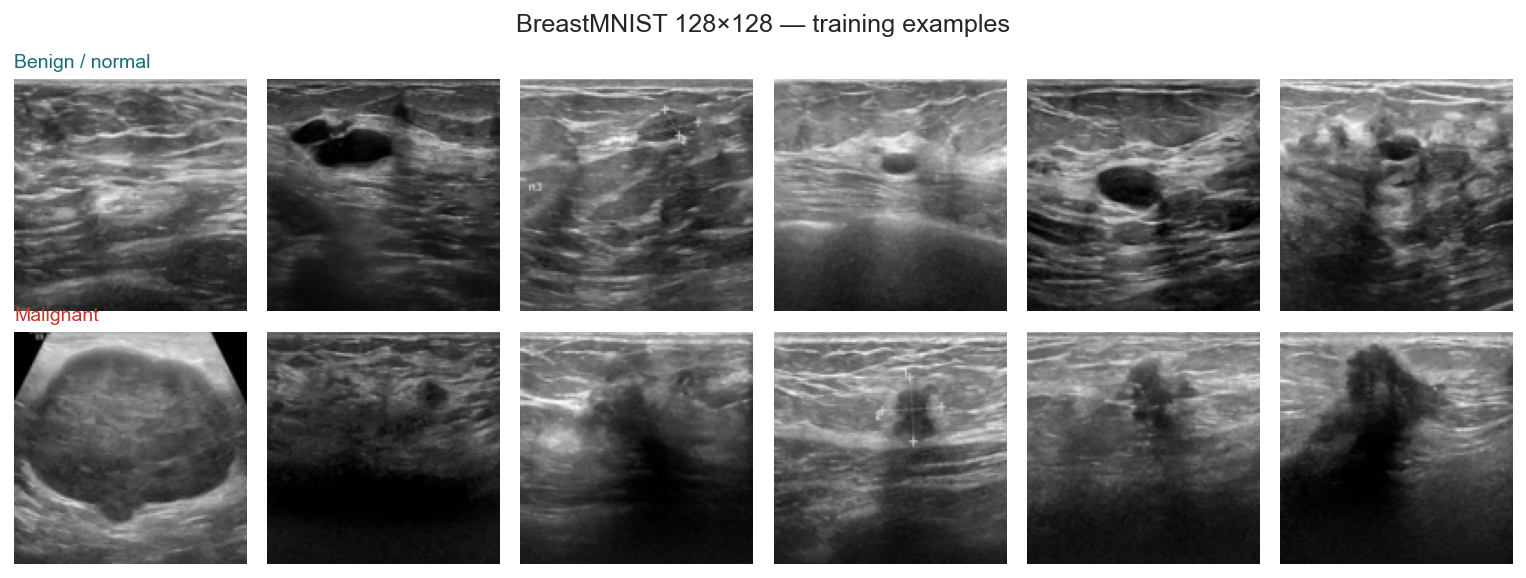
Malignant lesions on ultrasound often appear as darker (hypoechoic) regions with irregular margins and posterior shadowing. Benign cysts and fibroadenomas tend to be more oval and sharply bounded. At 128×128 those cues are still visible, but measurement crosshairs from the original scans remain in some frames — a shortcut a model could cheat with.

from IPython.display import Image, display
display(Image(str(FIG / '01_class_montage.png')))

Mean images

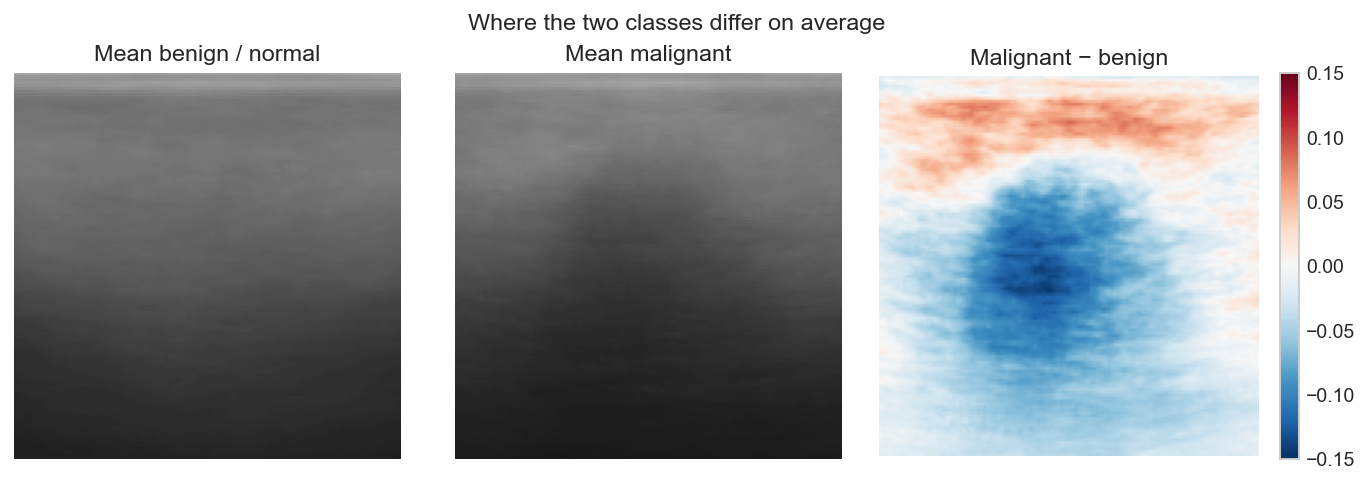
Averaging every training example of each class highlights where they differ on average.

display(Image(str(FIG / '01_mean_images.png')))

Intensity distributions

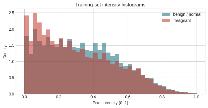
If malignant patches are systematically darker, a one-pixel statistic already carries signal — which is why the later random forest includes intensity summaries alongside HOG and LBP.

fig, ax = plt.subplots(figsize=(7.2, 3.8))
for cls, colour, label in [(0, '#1a6b7a', 'benign / normal'), (1, '#c0392b', 'malignant')]:
    pix = SPLITS['train']['images'][SPLITS['train']['labels'] == cls].ravel()
    ax.hist(pix, bins=40, density=True, alpha=0.55, color=colour, label=label)
ax.set_xlabel('Pixel intensity (0–1)')
ax.set_ylabel('Density')
ax.set_title('Training-set intensity histograms')
ax.legend(frameon=False)
plt.tight_layout()
plt.show()

Attribution

Yang et al., MedMNIST v2, Scientific Data (2023). Source images: Al-Dhabyani et al., Dataset of breast ultrasound images, Data in Brief (2020). See data/README.md.

---

Navigation: ← Previous: Project Overview | Next: Classical Models →