Partition

This chapter implements the Nystuen–Dacey dominant-flow algorithm in R: for each origin TTWA, follow the largest outward flow until a regional anchor (terminal node) is reached, then label every node by its anchor.

Previous: Flows
Next: Final map

suppressPackageStartupMessages({
  library(tidyverse)
  library(sf)
  library(ggraph)
  library(ggplot2)
  library(tidygraph)
  library(sfnetworks)
  library(here)
})

proj_dir <- here::here("projects", "uk-urban-systems-network")
data_dir <- file.path(proj_dir, "data")
fig_dir <- file.path(proj_dir, "figures")
dir.create(data_dir, recursive = TRUE, showWarnings = FALSE)
dir.create(fig_dir, recursive = TRUE, showWarnings = FALSE)

network_bundle <- readRDS(file.path(data_dir, "sfnetwork_graph.rds"))
g_net <- network_bundle$graph
nodes_sf <- network_bundle$nodes_sf
od_ttwa_pairs <- readRDS(file.path(data_dir, "od_ttwa_pairs.rds"))
ttwa_centroids <- readRDS(file.path(data_dir, "ttwa_centroids.rds"))

Nystuen–Dacey dominant-flow partition

#' Dominant-flow / nodal regions (Route B — not modularity clustering)
#'
#' For each origin, assign the destination with the largest outflow (excluding self).
#' Walk chains until a terminal node: one whose dominant partner sends less inflow
#' than the node's total inflow (regional anchor).
nystuen_dacey_dominant_flow <- function(edges, node_ids) {
  all_edges <- edges |> filter(origin_ttwa != dest_ttwa)

  dominant <- all_edges |>
    group_by(origin_ttwa) |>
    slice_max(flow, n = 1, with_ties = FALSE) |>
    ungroup() |>
    transmute(ttwa = origin_ttwa, partner = dest_ttwa, dominant_flow = flow)

  inflow <- all_edges |>
    group_by(dest_ttwa) |>
    summarise(inflow = sum(flow), .groups = "drop") |>
    rename(ttwa = dest_ttwa)

  node_set <- unique(node_ids)
  total_in <- inflow |>
    right_join(tibble(ttwa = node_set), by = "ttwa") |>
    mutate(inflow = replace_na(inflow, 0))

  is_terminal <- function(ttwa) {
    row <- dominant |> filter(ttwa == !!ttwa)
    if (nrow(row) == 0) return(TRUE)
    partner <- row$partner[1]
    partner_in <- total_in |> filter(ttwa == partner) |> pull(inflow)
    if (length(partner_in) == 0) partner_in <- 0
    self_in <- total_in |> filter(ttwa == !!ttwa) |> pull(inflow)
    partner_in < self_in
  }

  anchor_of <- function(ttwa) {
    visited <- character()
    current <- ttwa
  repeat {
      if (is_terminal(current)) return(current)
      nxt <- dominant |> filter(ttwa == current) |> pull(partner)
      if (length(nxt) == 0 || nxt[1] %in% visited) return(current)
      visited <- c(visited, current)
      current <- nxt[1]
    }
  }

  tibble(
    ttwa11cd = node_set,
    anchor_ttwa = vapply(node_set, anchor_of, character(1))
  ) |>
    mutate(region_id = as.integer(factor(anchor_ttwa)))
}

node_ids <- unique(c(od_ttwa_pairs$origin_ttwa, od_ttwa_pairs$dest_ttwa))
partition_labels <- nystuen_dacey_dominant_flow(od_ttwa_pairs, node_ids)

saveRDS(partition_labels, file.path(data_dir, "partition_labels.rds"))

Regional anchors

anchor_summary <- partition_labels |>
  count(anchor_ttwa, name = "n_members") |>
  arrange(desc(n_members))

print(anchor_summary)

# A tibble: 41 × 2
   anchor_ttwa n_members
   <chr>           <int>
 1 E30000234          32
 2 E30000229          12
 3 E30000239           9
 4 S22000065           9
 5 S22000068           9
 6 E30000169           8
 7 E30000206           8
 8 E30000248           7
 9 E30000110           6
10 E30000245           6
# ℹ 31 more rows

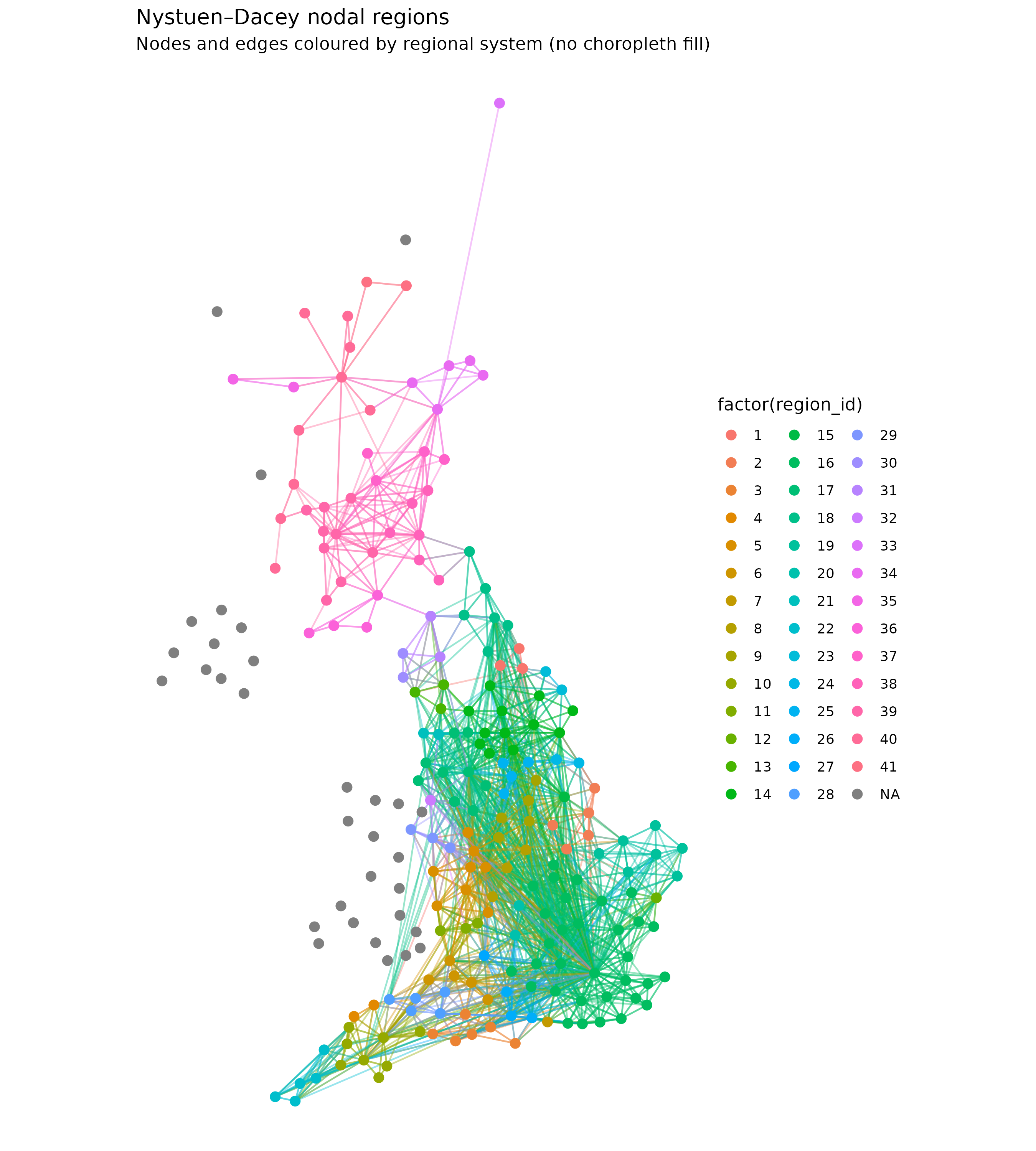
Partition map (nodes and edges only)

Interactive partition map

Pan and zoom the UK map below; click a TTWA for its regional system. Commuting links show flows ≥ 100 (display subset). Toggle country layers in the control panel.

suppressPackageStartupMessages({
  library(leaflet)
  library(htmlwidgets)
  library(htmltools)
  library(IRdisplay)
})

source(file.path(proj_dir, "R", "map_interactive.R"))

ttwa_boundaries <- readRDS(file.path(data_dir, "ttwa_boundaries.rds"))
edge_segments <- prepare_edge_segments(od_ttwa_pairs, ttwa_centroids, min_flow = 100L)

map_part <- leaflet_ttwa_network(
  ttwa_boundaries,
  partition_labels,
  edge_segments,
  mode = "partition"
)

include_leaflet_map(map_part, "UK nodal regions (interactive)", "06_partition_interactive")

Input to asJSON(keep_vec_names=TRUE) is a named vector. In a future version of jsonlite, this option will not be supported, and named vectors will be translated into arrays instead of objects. If you want JSON object output, please use a named list instead. See ?toJSON.

Input to asJSON(keep_vec_names=TRUE) is a named vector. In a future version of jsonlite, this option will not be supported, and named vectors will be translated into arrays instead of objects. If you want JSON object output, please use a named list instead. See ?toJSON.

Input to asJSON(keep_vec_names=TRUE) is a named vector. In a future version of jsonlite, this option will not be supported, and named vectors will be translated into arrays instead of objects. If you want JSON object output, please use a named list instead. See ?toJSON.

Input to asJSON(keep_vec_names=TRUE) is a named vector. In a future version of jsonlite, this option will not be supported, and named vectors will be translated into arrays instead of objects. If you want JSON object output, please use a named list instead. See ?toJSON.

Input to asJSON(keep_vec_names=TRUE) is a named vector. In a future version of jsonlite, this option will not be supported, and named vectors will be translated into arrays instead of objects. If you want JSON object output, please use a named list instead. See ?toJSON.

Input to asJSON(keep_vec_names=TRUE) is a named vector. In a future version of jsonlite, this option will not be supported, and named vectors will be translated into arrays instead of objects. If you want JSON object output, please use a named list instead. See ?toJSON.

Warning message in file(file, ifelse(append, "a", "w")):
“cannot open file '/Users/areeslindley/Documents/Git_repositories/projects-website/.cursor/debug-0556ee.log': No such file or directory”

UK nodal regions (interactive)

nodes_lab <- ttwa_centroids |>
  left_join(partition_labels, by = "ttwa11cd") |>
  mutate(name = ttwa11cd)

coords <- st_coordinates(nodes_lab)
nodes_plot <- nodes_lab |>
  st_drop_geometry() |>
  mutate(x = coords[, 1], y = coords[, 2])

edges_plot <- od_ttwa_pairs |>
  left_join(partition_labels |> rename(from = ttwa11cd), by = c("origin_ttwa" = "from"))

g_part <- tbl_graph(
  nodes = nodes_plot,
  edges = edges_plot |> transmute(from = origin_ttwa, to = dest_ttwa, flow, region_id),
  directed = TRUE
)

layout_part <- create_layout(g_part, layout = "manual", x = nodes_plot$x, y = nodes_plot$y)

p_part <- ggraph(layout_part) +
  geom_edge_link(aes(colour = factor(region_id)), alpha = 0.4, show.legend = FALSE) +
  geom_node_point(aes(colour = factor(region_id)), size = 2.5) +
  coord_sf(crs = sf::st_crs(ttwa_centroids), default_crs = sf::st_crs(ttwa_centroids)) +
  labs(
    title = "Nystuen–Dacey nodal regions",
    subtitle = "Nodes and edges coloured by regional system (no choropleth fill)"
  ) +
  theme_void()

fig_part <- file.path(fig_dir, "06_partition_map.png")
ggsave(fig_part, p_part, width = 9, height = 10, dpi = 300)
invisible(fig_part)

---

Next: Final map →