Simple Exponential Smoothing (SES)#
Navigation: ← Previous: Introduction | Next: Holt-Winters →
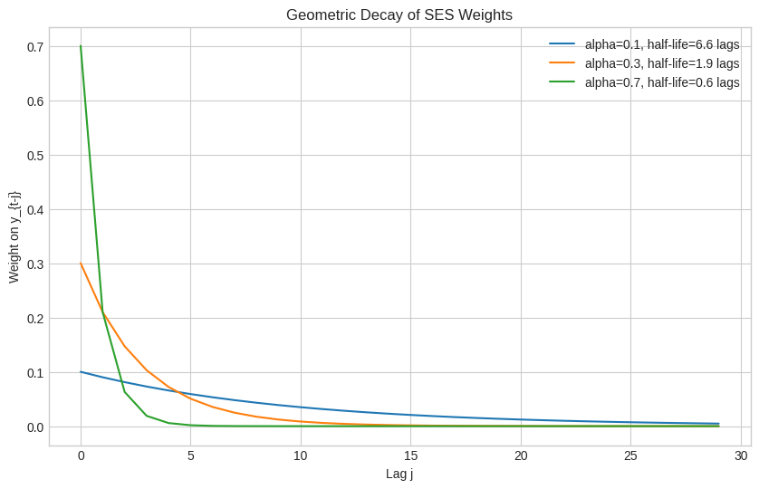
Simple Exponential Smoothing updates a level estimate with geometrically decaying weights. It is appropriate for series without trend or seasonality after preprocessing.
from pathlib import Path
import pandas as pd
import numpy as np
import matplotlib.pyplot as plt
import warnings
warnings.filterwarnings('ignore')
plt.style.use('seaborn-v0_8-whitegrid')

DATA_DIR = Path('data')
if not DATA_DIR.exists():
    DATA_DIR = Path('projects/time-series-analysis/data')

def load_series(name):
    """Load a bundled CSV as a DatetimeIndex Series."""
    df = pd.read_csv(DATA_DIR / name, parse_dates=['date'])
    return df.set_index('date')['value'].sort_index()

def load_air_passengers():
    path = DATA_DIR / 'air_passengers.csv'
    if path.exists():
        return load_series('air_passengers.csv')
    from statsmodels.datasets import get_rdataset
    air = get_rdataset('AirPassengers', 'datasets').data
    s = air['value']
    s.index = pd.date_range('1949-01', periods=len(s), freq='MS')
    return s

def load_milk():
    path = DATA_DIR / 'monthly_milk.csv'
    if path.exists():
        return load_series('monthly_milk.csv')
    url = 'https://raw.githubusercontent.com/jbrownlee/Datasets/master/monthly-milk-production-pounds.csv'
    return pd.read_csv(url, index_col=0, parse_dates=True).squeeze()

def load_co2():
    from statsmodels.datasets import co2
    return co2.load().data.resample('MS').mean().ffill().squeeze()

def load_sunspots():
    from statsmodels.datasets import sunspots
    d = sunspots.load_pandas().data
    return d.set_index('YEAR')['SUNACTIVITY']

def load_retail():
    path = DATA_DIR / 'uk_retail_sales.csv'
    if path.exists():
        return load_series('uk_retail_sales.csv')
    raise FileNotFoundError('uk_retail_sales.csv not found in data/')
from scipy.optimize import minimize_scalar
from statsmodels.tsa.holtwinters import SimpleExpSmoothing
from statsmodels.tsa.arima.model import ARIMA
The SES Recurrence#
Expanded: \(\ell_t = \sum_{j=0}^{t-1} \alpha(1-\alpha)^j y_{t-j} + (1-\alpha)^t \ell_0\). Forecasts are flat: \(\hat{y}_{T+h|T} = \ell_T\).
# Weight profiles for different alpha values
alphas = [0.1, 0.3, 0.7]
lags = np.arange(30)
fig, ax = plt.subplots(figsize=(10, 6))
for a in alphas:
    weights = a * (1 - a) ** lags
    ax.plot(lags, weights, label=f'alpha={a}, half-life={np.log(0.5)/np.log(1-a):.1f} lags')
ax.set_xlabel('Lag j')
ax.set_ylabel('Weight on y_{t-j}')
ax.set_title('Geometric Decay of SES Weights')
ax.legend()
fig
Manual SSE Optimisation#
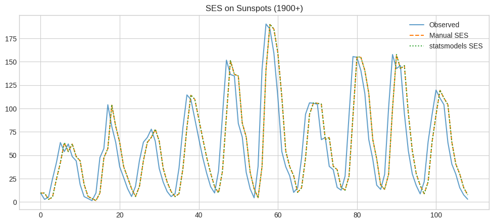
We minimise one-step-ahead sum of squared errors to estimate \(\alpha\).
def ses_forecast(y, alpha, l0=None):
    l0 = l0 if l0 is not None else y[0]
    level = l0
    preds = []
    for obs in y:
        preds.append(level)
        level = alpha * obs + (1 - alpha) * level
    return np.array(preds), level

def ses_sse(alpha, y):
    preds, _ = ses_forecast(y, alpha)
    return np.sum((y[1:] - preds[:-1]) ** 2)

spots = load_sunspots().astype(float)
# Use a stationary window (recent sunspot cycle)
y = spots.loc[1900:].values
result = minimize_scalar(ses_sse, bounds=(0.01, 0.99), method='bounded', args=(y,))
alpha_hat = result.x
print(f'Optimal alpha (manual): {alpha_hat:.4f}')
Optimal alpha (manual): 0.9900
# Compare manual vs statsmodels SES
model = SimpleExpSmoothing(y, initialization_method='estimated').fit(optimized=True)
print(f'Optimized alpha (statsmodels): {model.params["smoothing_level"]:.4f}')

manual_preds, _ = ses_forecast(y, alpha_hat)
fig, ax = plt.subplots(figsize=(12, 5))
ax.plot(y, label='Observed', alpha=0.7)
ax.plot(manual_preds, label='Manual SES', ls='--')
ax.plot(model.fittedvalues, label='statsmodels SES', ls=':')
ax.set_title('SES on Sunspots (1900+)')
ax.legend()
fig
Optimized alpha (statsmodels): 1.0000
ARIMA(0,1,1) Equivalence#
SES on differenced data is equivalent to ARIMA(0,1,1) with \(\theta = 1 - \alpha\).
milk = load_milk().values
alpha_m = minimize_scalar(ses_sse, bounds=(0.01, 0.99), method='bounded', args=(milk,)).x
arima = ARIMA(milk, order=(0, 1, 1)).fit()
params = arima.params
theta = params['ma.L1'] if hasattr(params, 'index') and 'ma.L1' in params.index else float(params[-1])
print(f'SES alpha: {alpha_m:.4f}  <=>  ARIMA theta: {theta:.4f}  (1-alpha = {1-alpha_m:.4f})')
SES alpha: 0.9900 <=> ARIMA theta: 202.9110 (1-alpha = 0.0100)
Key Takeaways#
Alpha controls memory: Higher \(\alpha\) reacts faster to shocks; lower \(\alpha\) gives smoother level estimates.
Flat forecasts: SES cannot extrapolate trend — inappropriate for Air Passengers without differencing.
ARIMA link: SES \(\equiv\) ARIMA(0,1,1) — connecting exponential smoothing to the Box-Jenkins framework.
Limitation: Assumes no trend or seasonality in the target series.
Navigation: ← Previous: Introduction | Next: Holt-Winters →