French Rugby Voronoi Analysis: Team Territories#
This notebook creates Voronoi diagrams showing the geographic territories of professional French rugby teams in Top 14 and Pro D2 leagues.
What is a Voronoi Diagram?#
A Voronoi diagram partitions a plane into regions based on proximity to a set of points. In this case, each region represents the area of France closest to a particular rugby team’s home stadium.
Objectives#
Load team location data (coordinates of stadiums)
Create Voronoi tessellation based on team locations
Visualize territories on a map of France
Analyze geographic patterns and territorial dominance
Generate insights about rugby’s geographic distribution in France
Introduction and Data Setup#
We’ll begin by importing the necessary libraries for geospatial analysis, visualization, and Voronoi tessellation. This project requires specialized geospatial libraries to handle coordinate systems, geometric operations, and map visualization.
# Geospatial analysis
import geopandas as gpd
from shapely.geometry import Point, Polygon
from shapely.ops import voronoi_diagram, nearest_points
import folium
from folium import plugins
from geovoronoi import voronoi_regions_from_coords, points_to_coords

# Data manipulation
import pandas as pd
import numpy as np

# Visualization
import matplotlib.pyplot as plt
import matplotlib.patches as mpatches
from matplotlib.colors import ListedColormap
import seaborn as sns

# Spatial algorithms
from scipy.spatial import Voronoi, voronoi_plot_2d

# Utilities
import warnings
import os
import requests
from io import BytesIO
import zipfile
warnings.filterwarnings('ignore')

# Check if running in CI environment
is_ci = os.environ.get('CI', 'false').lower() == 'true'

# Set visualization style
sns.set_context("notebook", font_scale=1.1)
sns.set_style("whitegrid")
plt.rcParams['figure.figsize'] = (12, 8)
plt.rcParams['figure.dpi'] = 100

# Set random seed for reproducibility
np.random.seed(42)

print("Libraries imported successfully!")
Libraries imported successfully!
Team Locations and Coordinates#
To create accurate Voronoi diagrams, we need the geographic coordinates (latitude and longitude) of each professional rugby team’s home stadium. These coordinates will serve as the “seeds” or “generators” for the Voronoi tessellation.
The data includes teams from:
Top 14: France’s premier professional rugby union league
Pro D2: The second-tier professional league
Each team’s location represents where fans would travel from to attend home matches, making this a natural application of proximity analysis.
# Team data with actual coordinates from French rugby leagues
# Coordinates are in (Latitude, Longitude) format

# Top 14 teams
top14_teams = {
    'Team': ['Toulouse', 'Toulon', 'La Rochelle', 'Bordeaux', 'Racing 92',
             'Stade Français', 'Clermont', 'Lyon', 'Castres', 'Montpellier',
             'Bayonne', 'Pau', 'Perpignan', 'Montauban'],
    'City': ['Toulouse', 'Toulon', 'La Rochelle', 'Bordeaux', 'Nanterre',
             'Paris', 'Clermont-Ferrand', 'Lyon', 'Castres', 'Montpellier',
             'Bayonne', 'Pau', 'Perpignan', 'Montauban'],
    'Latitude': [43.621, 43.125, 46.158, 44.829, 48.895,
                 48.844, 45.791, 45.724, 43.601, 43.590,
                 43.484, 43.303, 42.711, 44.017],
    'Longitude': [1.415, 5.934, -1.171, -0.598, 2.229,
                  2.252, 3.106, 4.832, 2.249, 3.861,
                  -1.486, -0.322, 2.894, 1.355],
    'League': ['Top 14'] * 14
}

# Pro D2 teams
prod2_teams = {
    'Team': ['Vannes', 'Brive', 'Biarritz', 'Agen', 'Colomiers',
             'Mont-de-Marsan', 'Dax', 'Béziers', 'Carcassonne', 'Oyonnax',
             'Grenoble', 'Aurillac', 'Valence Romans', 'Provence',
             'Nevers', 'Soyaux-Angoulême'],
    'City': ['Vannes', 'Brive-la-Gaillarde', 'Biarritz', 'Agen', 'Colomiers',
             'Mont-de-Marsan', 'Dax', 'Béziers', 'Carcassonne', 'Oyonnax',
             'Grenoble', 'Aurillac', 'Valence', 'Aix-en-Provence',
             'Nevers', 'Angoulême'],
    'Latitude': [47.662, 45.147, 43.476, 44.197, 43.611,
                 43.892, 43.712, 43.344, 43.210, 46.262,
                 45.178, 44.921, 44.931, 43.541,
                 46.993, 45.657],
    'Longitude': [-2.766, 1.526, -1.551, 0.622, 1.341,
                  -0.491, -1.051, 3.237, 2.350, 5.656,
                  5.742, 2.441, 4.901, 5.421,
                  3.146, 0.171],
    'League': ['Pro D2'] * 16
}

# Combine both leagues
teams_data = {
    'Team': top14_teams['Team'] + prod2_teams['Team'],
    'City': top14_teams['City'] + prod2_teams['City'],
    'Latitude': top14_teams['Latitude'] + prod2_teams['Latitude'],
    'Longitude': top14_teams['Longitude'] + prod2_teams['Longitude'],
    'League': top14_teams['League'] + prod2_teams['League']
}

teams_df = pd.DataFrame(teams_data)

# Create GeoDataFrame with Point geometries
geometry = [Point(xy) for xy in zip(teams_df['Longitude'], teams_df['Latitude'])]
teams_gdf = gpd.GeoDataFrame(teams_df, geometry=geometry, crs='EPSG:4326')

print(f"Loaded {len(teams_df)} teams")
print(f"\nLeague distribution:")
print(teams_df['League'].value_counts())
print(f"\nFirst few teams:")
display(teams_df.head())
Loaded 30 teams

League distribution:
League
Pro D2    16
Top 14    14
Name: count, dtype: int64

First few teams:
| Team | City | Latitude | Longitude | League | |
|---|---|---|---|---|---|
| 0 | Toulouse | Toulouse | 43.621 | 1.415 | Top 14 |
| 1 | Toulon | Toulon | 43.125 | 5.934 | Top 14 |
| 2 | La Rochelle | La Rochelle | 46.158 | -1.171 | Top 14 |
| 3 | Bordeaux | Bordeaux | 44.829 | -0.598 | Top 14 |
| 4 | Racing 92 | Nanterre | 48.895 | 2.229 | Top 14 |
Visualizing Team Locations#
Let’s first plot the team locations on a map to see their geographic distribution before creating the Voronoi diagram.
# Create a base map centered on France
# Note: Folium maps require JavaScript and may not render in all environments
# Skip interactive map generation in CI/build environments

if not is_ci:
    try:
        france_map = folium.Map(
            location=[46.5, 2.5],  # Center of France
            zoom_start=6,
            tiles='OpenStreetMap'
        )

        # Add team markers
        for idx, row in teams_df.iterrows():
            color = 'blue' if row['League'] == 'Top 14' else 'green'
            folium.CircleMarker(
                location=[row['Latitude'], row['Longitude']],
                radius=8,
                popup=f"{row['Team']} ({row['League']})",
                color=color,
                fill=True,
                fillColor=color,
                fillOpacity=0.7
            ).add_to(france_map)

        # Add legend
        legend_html = '''
        <div style="position: fixed; bottom: 50px; left: 50px; width: 150px;
                    background-color: white; z-index:9999; border:2px solid grey;
                    border-radius:5px; padding: 10px">
        <p><b>Legend</b></p>
        <p><span style="color:blue">●</span> Top 14</p>
        <p><span style="color:green">●</span> Pro D2</p>
        </div>
        '''
        france_map.get_root().html.add_child(folium.Element(legend_html))

        # Display map
        france_map
    except Exception as e:
        print(f"Note: Interactive map generation skipped ({e})")
        print("Team locations will be shown in the Voronoi diagrams below.")
else:
    print("Skipping interactive map generation in CI environment.")
    print("Team locations will be shown in the Voronoi diagrams below.")
Skipping interactive map generation in CI environment.
Team locations will be shown in the Voronoi diagrams below.
Observation: The map reveals a clear clustering of teams in southwestern France, particularly in the Occitanie and Nouvelle-Aquitaine regions. This aligns with rugby’s historical stronghold in France, where the sport has deep cultural roots. Northern France, despite having large population centers like Paris, has relatively fewer professional teams.
Voronoi Tessellation#
Now we’ll create the Voronoi diagram. The Voronoi tessellation will partition France into regions where each region contains all points closer to one team’s stadium than to any other. This effectively shows each team’s “territorial catchment area.”
# Load France boundary for accurate Voronoi clipping
# Using Natural Earth high-resolution data for better accuracy
# With robust error handling for CI environments

try:
    # Try to download Natural Earth data with timeout
    url = "https://naciscdn.org/naturalearth/10m/cultural/ne_10m_admin_0_countries.zip"
    print("Downloading France boundary data...")
    response = requests.get(url, timeout=30)
    response.raise_for_status()

    # Read from memory
    with zipfile.ZipFile(BytesIO(response.content)) as z:
        world = gpd.read_file(z)

    france = world[world.ADMIN == 'France'].to_crs(epsg=3857)  # Web Mercator for Voronoi

    # Clip to mainland France (exclude overseas territories)
    france = france.clip_by_rect(-600000, 5000000, 1200000, 6650000)
    france_boundary = france.geometry.union_all()
    print("✓ Loaded France boundary from Natural Earth")
except Exception as e:
    print(f"Could not load France boundary from Natural Earth: {e}")
    print("Using approximate bounding box instead...")
    # Fallback to bounding box
    france_bbox = Polygon([
        (-5.0, 42.0),  # Southwest
        (8.0, 42.0),   # Southeast
        (8.0, 51.0),   # Northeast
        (-5.0, 51.0),  # Northwest
        (-5.0, 42.0)   # Close polygon
    ])
    france_bbox_gdf = gpd.GeoDataFrame([1], geometry=[france_bbox], crs='EPSG:4326')
    france = france_bbox_gdf.to_crs('EPSG:3857')
    france_boundary = france.geometry.iloc[0]
    print("✓ Using bounding box as France boundary")

# Convert teams to Web Mercator (EPSG:3857) for Voronoi calculation
teams_gdf_projected = teams_gdf.to_crs('EPSG:3857')

# Ensure all points are inside the boundary (snap coastal points to land)
for idx, row in teams_gdf_projected.iterrows():
    if not row.geometry.within(france_boundary):
        # Find nearest point on boundary
        p1, p2 = nearest_points(france_boundary, row.geometry)
        teams_gdf_projected.at[idx, 'geometry'] = p1

# Extract coordinates for Voronoi calculation
coords = points_to_coords(teams_gdf_projected.geometry)

print(f"✓ Prepared {len(coords)} team locations for Voronoi tessellation")
Downloading France boundary data...
Could not load France boundary from Natural Earth: ZipFile.read() missing 1 required positional argument: 'name'
Using approximate bounding box instead...
✓ Using bounding box as France boundary
✓ Prepared 30 team locations for Voronoi tessellation
Creating Bounded Voronoi Regions#
The raw Voronoi diagram extends infinitely. We’ll use the geovoronoi library to create Voronoi regions that are automatically clipped to France’s boundaries. This ensures accurate territorial regions that respect the country’s coastline and borders.
# Generate Voronoi regions clipped to France boundary
region_polys, region_pts = voronoi_regions_from_coords(coords, france_boundary)

# Create GeoDataFrame with Voronoi regions
voronoi_polygons = []
team_names = []

for region_id, poly in region_polys.items():
    team_idx = region_pts[region_id][0]
    team_name = teams_df.iloc[team_idx]['Team']
    voronoi_polygons.append(poly)
    team_names.append(team_name)

# Create GeoDataFrame
voronoi_gdf = gpd.GeoDataFrame({
    'Team': team_names,
    'geometry': voronoi_polygons
}, crs=teams_gdf_projected.crs)

# Merge with team information
voronoi_gdf = voronoi_gdf.merge(
    teams_df[['Team', 'League', 'City']],
    on='Team',
    how='left'
)

# Calculate territory areas
voronoi_gdf['Area_km2'] = voronoi_gdf.geometry.area / 1e6  # Convert from m² to km²

print(f"✓ Created {len(voronoi_gdf)} bounded Voronoi regions")
print(f"✓ Total territory area: {voronoi_gdf['Area_km2'].sum():.0f} km²")
display(voronoi_gdf.head())
✓ Created 30 bounded Voronoi regions
✓ Total territory area: 2113299 km²
| Team | geometry | League | City | Area_km2 | |
|---|---|---|---|---|---|
| 0 | Stade Français | POLYGON ((624761.281 6199641.786, 68740.14 601... | Top 14 | Paris | 129893.320004 |
| 1 | Racing 92 | POLYGON ((673717.263 6621293.723, 890555.926 6... | Top 14 | Nanterre | 330294.438966 |
| 2 | Vannes | POLYGON ((-203250.612 6621293.723, -35222.643 ... | Pro D2 | Vannes | 353880.923054 |
| 3 | Lyon | POLYGON ((573566.486 5675394.714, 437682.488 5... | Top 14 | Lyon | 25503.531558 |
| 4 | Oyonnax | POLYGON ((489187.393 5879962.592, 624761.281 6... | Pro D2 | Oyonnax | 184285.713276 |
Generating Separate League Diagrams#
Let’s create separate Voronoi diagrams for Top 14 and Pro D2 leagues to better visualize each league’s territorial distribution. These will be saved as images for display on the project overview page.
import os
import contextily as cx

# Create images directory if it doesn't exist
os.makedirs('images', exist_ok=True)

# Function to create Voronoi diagram for a specific league
def create_league_voronoi(league_name, teams_subset, france_boundary):
    """Create Voronoi diagram for a specific league"""
    # Create GeoDataFrame for this league
    geometry = [Point(xy) for xy in zip(teams_subset['Longitude'], teams_subset['Latitude'])]
    league_gdf = gpd.GeoDataFrame(teams_subset, geometry=geometry, crs='EPSG:4326')
    league_gdf = league_gdf.to_crs('EPSG:3857')

    # Ensure all points are inside boundary
    for idx, row in league_gdf.iterrows():
        if not row.geometry.within(france_boundary):
            p1, p2 = nearest_points(france_boundary, row.geometry)
            league_gdf.at[idx, 'geometry'] = p1

    # Generate Voronoi regions
    coords = points_to_coords(league_gdf.geometry)
    region_polys, region_pts = voronoi_regions_from_coords(coords, france_boundary)

    # Create GeoDataFrame
    voronoi_polygons = []
    team_names = []

    for region_id, poly in region_polys.items():
        team_idx = region_pts[region_id][0]
        team_name = teams_subset.iloc[team_idx]['Team']
        voronoi_polygons.append(poly)
        team_names.append(team_name)

    voronoi_gdf = gpd.GeoDataFrame({
        'Team': team_names,
        'geometry': voronoi_polygons
    }, crs=league_gdf.crs)

    voronoi_gdf = voronoi_gdf.merge(
        teams_subset[['Team', 'City']],
        on='Team',
        how='left'
    )

    return voronoi_gdf, league_gdf

# Create separate diagrams for Top 14 and Pro D2
top14_teams_df = teams_df[teams_df['League'] == 'Top 14'].copy()
prod2_teams_df = teams_df[teams_df['League'] == 'Pro D2'].copy()

print("Creating Top 14 Voronoi diagram...")
top14_voronoi, top14_points = create_league_voronoi('Top 14', top14_teams_df, france_boundary)
print(f"✓ Top 14: {len(top14_voronoi)} regions")

print("\nCreating Pro D2 Voronoi diagram...")
prod2_voronoi, prod2_points = create_league_voronoi('Pro D2', prod2_teams_df, france_boundary)
print(f"✓ Pro D2: {len(prod2_voronoi)} regions")

# Convert to WGS84 for visualization
top14_voronoi_wgs84 = top14_voronoi.to_crs('EPSG:4326')
top14_points_wgs84 = top14_points.to_crs('EPSG:4326')
prod2_voronoi_wgs84 = prod2_voronoi.to_crs('EPSG:4326')
prod2_points_wgs84 = prod2_points.to_crs('EPSG:4326')

# Load France boundary in WGS84 for plotting
# Re-load France boundary for visualization (in case it wasn't loaded earlier)
try:
    url = "https://naciscdn.org/naturalearth/10m/cultural/ne_10m_admin_0_countries.zip"
    world_viz = gpd.read_file(url)
    france_viz = world_viz[world_viz.ADMIN == 'France'].to_crs(epsg=4326)
    france_viz = france_viz.clip_by_rect(-5.5, 41.0, 9.5, 51.5)
    france_wgs84 = france_viz
    print("✓ Loaded France boundary for visualization")
except Exception as e:
    print(f"Using simple bounding box for visualization: {e}")
    # Fallback: create a simple France outline
    france_bbox_wgs84 = Polygon([
        (-5.0, 42.0),  # Southwest
        (8.0, 42.0),   # Southeast
        (8.0, 51.0),   # Northeast
        (-5.0, 51.0),  # Northwest
        (-5.0, 42.0)   # Close polygon
    ])
    france_wgs84 = gpd.GeoDataFrame([1], geometry=[france_bbox_wgs84], crs='EPSG:4326')

# Create Top 14 diagram
fig, ax = plt.subplots(figsize=(14, 12))
france_wgs84.plot(ax=ax, color='none', edgecolor='black', linewidth=1.5, zorder=3)

# Plot Top 14 Voronoi regions
for idx, row in top14_voronoi_wgs84.iterrows():
    gpd.GeoSeries([row.geometry]).plot(
        ax=ax,
        facecolor='#1f77b4',
        alpha=0.5,
        edgecolor='white',
        linewidth=1.5,
        zorder=1
    )

# Plot Top 14 team locations
for idx, row in top14_points_wgs84.iterrows():
    team_name = row['Team']
    ax.plot(
        row.geometry.x,
        row.geometry.y,
        marker='o',
        markersize=12,
        color='white',
        markeredgecolor='#1f77b4',
        markeredgewidth=2,
        zorder=4
    )
    ax.annotate(
        team_name,
        (row.geometry.x, row.geometry.y),
        fontsize=9,
        ha='center',
        va='bottom',
        bbox=dict(boxstyle='round,pad=0.3', facecolor='white', alpha=0.8, edgecolor='#1f77b4'),
        zorder=5
    )

ax.set_xlim(-5.5, 9.5)
ax.set_ylim(41.5, 51.5)
ax.set_title('Top 14: Team Territories', fontsize=18, fontweight='bold', pad=20)
ax.set_axis_off()

# Add basemap
try:
    ax_3857 = ax
    # Convert axes limits to Web Mercator for basemap
    xlim = ax.get_xlim()
    ylim = ax.get_ylim()
    # Note: contextily works better with projected coordinates, but we'll skip it for now
    # to avoid coordinate system issues
except:
    pass

plt.tight_layout()
plt.savefig('images/top14_voronoi.png', dpi=150, bbox_inches='tight', facecolor='white')
plt.close()
print("✓ Saved: images/top14_voronoi.png")

# Create Pro D2 diagram
fig, ax = plt.subplots(figsize=(14, 12))
france_wgs84.plot(ax=ax, color='none', edgecolor='black', linewidth=1.5, zorder=3)

# Plot Pro D2 Voronoi regions
for idx, row in prod2_voronoi_wgs84.iterrows():
    gpd.GeoSeries([row.geometry]).plot(
        ax=ax,
        facecolor='#2ca02c',
        alpha=0.5,
        edgecolor='white',
        linewidth=1.5,
        zorder=1
    )

# Plot Pro D2 team locations
for idx, row in prod2_points_wgs84.iterrows():
    team_name = row['Team']
    ax.plot(
        row.geometry.x,
        row.geometry.y,
        marker='o',
        markersize=12,
        color='white',
        markeredgecolor='#2ca02c',
        markeredgewidth=2,
        zorder=4
    )
    ax.annotate(
        team_name,
        (row.geometry.x, row.geometry.y),
        fontsize=9,
        ha='center',
        va='bottom',
        bbox=dict(boxstyle='round,pad=0.3', facecolor='white', alpha=0.8, edgecolor='#2ca02c'),
        zorder=5
    )

ax.set_xlim(-5.5, 9.5)
ax.set_ylim(41.5, 51.5)
ax.set_title('Pro D2: Team Territories', fontsize=18, fontweight='bold', pad=20)
ax.set_axis_off()

plt.tight_layout()
plt.savefig('images/prod2_voronoi.png', dpi=150, bbox_inches='tight', facecolor='white')
plt.close()
print("✓ Saved: images/prod2_voronoi.png")

print("\n✓ Both league diagrams saved successfully!")
Creating Top 14 Voronoi diagram...
✓ Top 14: 14 regions

Creating Pro D2 Voronoi diagram...
✓ Pro D2: 16 regions
✓ Loaded France boundary for visualization
✓ Saved: images/top14_voronoi.png
✓ Saved: images/prod2_voronoi.png

✓ Both league diagrams saved successfully!
Visualization#
Now we’ll create comprehensive visualizations showing the Voronoi territories. We’ll use both static matplotlib plots and interactive Folium maps to provide different perspectives on the geographic distribution.
# Create color map based on league
league_colors = {'Top 14': '#1f77b4', 'Pro D2': '#2ca02c'}

# Convert back to WGS84 for static visualization
voronoi_gdf_wgs84_static = voronoi_gdf.to_crs('EPSG:4326')
teams_gdf_wgs84_static = teams_gdf_projected.to_crs('EPSG:4326')

# Create static plot
fig, ax = plt.subplots(figsize=(14, 10))

# Plot Voronoi regions
for idx, row in voronoi_gdf_wgs84_static.iterrows():
    color = league_colors.get(row['League'], 'gray')
    gpd.GeoSeries([row.geometry]).plot(
        ax=ax,
        color=color,
        alpha=0.4,
        edgecolor='black',
        linewidth=1.5
    )

# Plot team locations
for idx, row in teams_gdf_wgs84_static.iterrows():
    color = league_colors.get(teams_df.iloc[idx]['League'], 'gray')
    ax.plot(
        row.geometry.x,
        row.geometry.y,
        marker='o',
        markersize=10,
        color=color,
        markeredgecolor='black',
        markeredgewidth=1.5,
        label=row['Team'] if idx == 0 else ""
    )

# Add team labels
for idx, row in teams_gdf_wgs84_static.iterrows():
    ax.annotate(
        row['Team'],
        (row.geometry.x, row.geometry.y),
        fontsize=8,
        ha='center',
        va='bottom',
        bbox=dict(boxstyle='round,pad=0.3', facecolor='white', alpha=0.7, edgecolor='none')
    )

ax.set_xlabel('Longitude', fontsize=12)
ax.set_ylabel('Latitude', fontsize=12)
ax.set_title('French Rugby Team Territories: Voronoi Diagram', fontsize=16, fontweight='bold', pad=20)

# Create custom legend
top14_patch = mpatches.Patch(color='#1f77b4', alpha=0.4, label='Top 14 Territory')
prod2_patch = mpatches.Patch(color='#2ca02c', alpha=0.4, label='Pro D2 Territory')
top14_marker = plt.Line2D([0], [0], marker='o', color='w', markerfacecolor='#1f77b4',
                          markersize=10, markeredgecolor='black', markeredgewidth=1.5, label='Top 14 Team')
prod2_marker = plt.Line2D([0], [0], marker='o', color='w', markerfacecolor='#2ca02c',
                          markersize=10, markeredgecolor='black', markeredgewidth=1.5, label='Pro D2 Team')

ax.legend(handles=[top14_patch, prod2_patch, top14_marker, prod2_marker],
          loc='upper right', fontsize=10)

ax.grid(True, alpha=0.3)
plt.tight_layout()
plt.show()
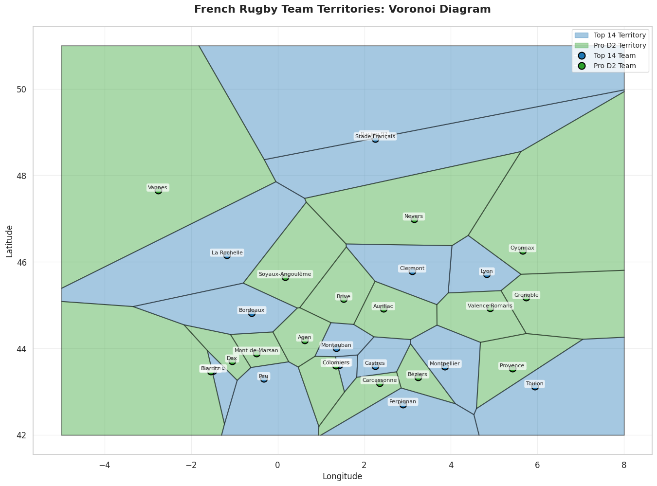
Key Observations from the Voronoi Diagram:
Southwestern Dominance: Teams in the southwest (Toulouse, Castres, Montpellier, etc.) control large territorial regions, reflecting rugby’s traditional heartland.
Sparse Northern Coverage: Despite Paris having teams (Racing 92, Stade Français), the northern regions show much larger territories per team, indicating fewer teams relative to the geographic area.
Coastal Clustering: Many teams are located along the Atlantic coast (La Rochelle, Bordeaux, Bayonne), creating interesting territorial boundaries.
Territorial Size Variation: Some teams like Toulouse and Clermont have very large territories, while teams in densely populated areas have smaller, more compact territories.
Interactive Map#
Let’s create an interactive map that allows users to explore the territories in detail.
# Convert Voronoi regions back to WGS84 for Folium
voronoi_gdf_wgs84 = voronoi_gdf.to_crs('EPSG:4326')
teams_gdf_wgs84 = teams_gdf_projected.to_crs('EPSG:4326')

# Create enhanced interactive map with Voronoi regions
interactive_map = folium.Map(
    location=[46.5, 2.5],
    zoom_start=6,
    tiles='OpenStreetMap',
    min_zoom=5,
    max_zoom=10
)

# Add Voronoi regions with enhanced interactivity
for idx, row in voronoi_gdf_wgs84.iterrows():
    color = league_colors.get(row['League'], 'gray')
    area = row.get('Area_km2', 0)

    # Create a style function that highlights on hover
    def make_style_function(team_color, team_name):
        def style_function(feature):
            return {
                'fillColor': team_color,
                'color': 'black',
                'weight': 2,
                'fillOpacity': 0.5,
                'opacity': 0.8
            }
        return style_function

    # Create interactive tooltip with territory information
    tooltip_html = f"""
    <div style="font-family: Arial, sans-serif;">
        <h4 style="margin: 5px 0; color: {color};">{row['Team']}</h4>
        <p style="margin: 2px 0;"><strong>League:</strong> {row['League']}</p>
        <p style="margin: 2px 0;"><strong>City:</strong> {row['City']}</p>
        <p style="margin: 2px 0;"><strong>Territory:</strong> {area:,.0f} km²</p>
        <p style="margin: 5px 0 0 0; font-size: 11px; color: #666;">Click for details</p>
    </div>
    """

    # Create detailed popup
    popup_html = f"""
    <div style="font-family: Arial, sans-serif; min-width: 200px;">
        <h3 style="margin: 0 0 10px 0; color: {color}; border-bottom: 2px solid {color}; padding-bottom: 5px;">
            {row['Team']}
        </h3>
        <table style="width: 100%; border-collapse: collapse;">
            <tr>
                <td style="padding: 5px; font-weight: bold;">League:</td>
                <td style="padding: 5px;">{row['League']}</td>
            </tr>
            <tr>
                <td style="padding: 5px; font-weight: bold;">City:</td>
                <td style="padding: 5px;">{row['City']}</td>
            </tr>
            <tr>
                <td style="padding: 5px; font-weight: bold;">Territory Area:</td>
                <td style="padding: 5px;">{area:,.0f} km²</td>
            </tr>
        </table>
        <p style="margin: 10px 0 0 0; font-size: 11px; color: #666; font-style: italic;">
            This region represents all points in France closest to {row['Team']}'s home stadium.
        </p>
    </div>
    """

    # Add Voronoi region with interactivity
    folium.GeoJson(
        row.geometry.__geo_interface__,
        style_function=make_style_function(color, row['Team']),
        tooltip=folium.Tooltip(tooltip_html, sticky=True),
        popup=folium.Popup(popup_html, max_width=300),
        highlight_function=lambda feature: {
            'fillOpacity': 0.8,
            'weight': 3,
            'color': 'white'
        }
    ).add_to(interactive_map)

# Add team location markers with custom icons
for idx, row in teams_gdf_wgs84.iterrows():
    team_info = teams_df.iloc[idx]
    color = league_colors.get(team_info['League'], 'gray')

    # Create custom icon
    icon_color = 'blue' if team_info['League'] == 'Top 14' else 'green'

    folium.CircleMarker(
        location=[row.geometry.y, row.geometry.x],
        radius=10,
        popup=folium.Popup(
            f"<b>{team_info['Team']}</b><br>"
            f"League: {team_info['League']}<br>"
            f"City: {team_info['City']}<br>"
            f"<em>Home Stadium Location</em>",
            max_width=200
        ),
        tooltip=f"{team_info['Team']} ({team_info['League']})",
        color='white',
        fillColor=color,
        fill=True,
        fillOpacity=0.9,
        weight=2.5
    ).add_to(interactive_map)

# Add enhanced legend with statistics
total_teams = len(teams_df)
top14_count = len(teams_df[teams_df['League'] == 'Top 14'])
prod2_count = len(teams_df[teams_df['League'] == 'Pro D2'])

legend_html = f'''
<div style="position: fixed; bottom: 50px; left: 50px; width: 220px;
            background-color: white; z-index:9999; border:2px solid #333;
            border-radius:8px; padding: 15px; font-family: Arial, sans-serif; box-shadow: 0 2px 8px rgba(0,0,0,0.2);">
<p style="margin:0 0 10px 0; font-weight:bold; font-size:14px; border-bottom: 2px solid #333; padding-bottom: 5px;">
    French Rugby Territories
</p>
<p style="margin:5px 0; font-size:12px;"><span style="color:#1f77b4; font-size:18px;">■</span> <strong>Top 14</strong> ({top14_count} teams)</p>
<p style="margin:5px 0; font-size:12px;"><span style="color:#2ca02c; font-size:18px;">■</span> <strong>Pro D2</strong> ({prod2_count} teams)</p>
<p style="margin:10px 0 0 0; font-size:11px; color:#666; border-top: 1px solid #ddd; padding-top: 8px;">
    <strong>Total:</strong> {total_teams} professional teams<br>
    Hover over regions for details
</p>
</div>
'''
interactive_map.get_root().html.add_child(folium.Element(legend_html))

# Add fullscreen button
plugins.Fullscreen().add_to(interactive_map)

# Add measure tool
plugins.MeasureControl().add_to(interactive_map)

# Display map
print("Interactive Voronoi Map:")
print("=" * 60)
print("• Hover over territories to see team information")
print("• Click on regions for detailed popups")
print("• Use the measure tool to calculate distances")
print("• Zoom and pan to explore different regions")
print("=" * 60)
interactive_map
Interactive Voronoi Map:
============================================================
• Hover over territories to see team information
• Click on regions for detailed popups
• Use the measure tool to calculate distances
• Zoom and pan to explore different regions
============================================================
Analysis and Insights#
Let’s quantify the territorial distribution by calculating the area of each team’s Voronoi region. This will help us identify which teams have the largest and smallest territories.
# Area already calculated during Voronoi creation
# Sort by area
territory_analysis = voronoi_gdf[['Team', 'League', 'City', 'Area_km2']].sort_values(
    'Area_km2',
    ascending=False
)

print("Territory Size Analysis")
print("="*60)
print(f"\nTotal territory covered: {voronoi_gdf['Area_km2'].sum():.0f} km²")
print(f"Average territory size: {voronoi_gdf['Area_km2'].mean():.0f} km²")
print(f"Median territory size: {voronoi_gdf['Area_km2'].median():.0f} km²")

print("\n" + "="*60)
print("Largest Territories:")
print("="*60)
display(territory_analysis.head(5))

print("\n" + "="*60)
print("Smallest Territories:")
print("="*60)
display(territory_analysis.tail(5))

# Visualize territory sizes
fig, ax = plt.subplots(figsize=(12, 6))
colors = [league_colors.get(league, 'gray') for league in territory_analysis['League']]
bars = ax.barh(range(len(territory_analysis)), territory_analysis['Area_km2'], color=colors, alpha=0.7)
ax.set_yticks(range(len(territory_analysis)))
ax.set_yticklabels(territory_analysis['Team'], fontsize=9)
ax.set_xlabel('Territory Area (km²)', fontsize=12)
ax.set_title('Territory Size by Team', fontsize=14, fontweight='bold')
ax.grid(True, alpha=0.3, axis='x')

# Add value labels
for i, (idx, row) in enumerate(territory_analysis.iterrows()):
    ax.text(row['Area_km2'] + 1000, i, f"{row['Area_km2']:.0f}",
            va='center', fontsize=8)

plt.tight_layout()
plt.show()
Territory Size Analysis
============================================================

Total territory covered: 2113299 km²
Average territory size: 70443 km²
Median territory size: 33572 km²

============================================================
Largest Territories:
============================================================
| Team | League | City | Area_km2 | |
|---|---|---|---|---|
| 2 | Vannes | Pro D2 | Vannes | 353880.923054 |
| 1 | Racing 92 | Top 14 | Nanterre | 330294.438966 |
| 4 | Oyonnax | Pro D2 | Oyonnax | 184285.713276 |
| 12 | Biarritz | Pro D2 | Biarritz | 169095.209750 |
| 0 | Stade Français | Top 14 | Paris | 129893.320004 |
============================================================
Smallest Territories:
============================================================
| Team | League | City | Area_km2 | |
|---|---|---|---|---|
| 14 | Dax | Pro D2 | Dax | 13082.428855 |
| 19 | Montauban | Top 14 | Montauban | 12554.758778 |
| 13 | Mont-de-Marsan | Pro D2 | Mont-de-Marsan | 12312.543273 |
| 11 | Bayonne | Top 14 | Bayonne | 7639.764155 |
| 18 | Toulouse | Top 14 | Toulouse | 4847.908774 |
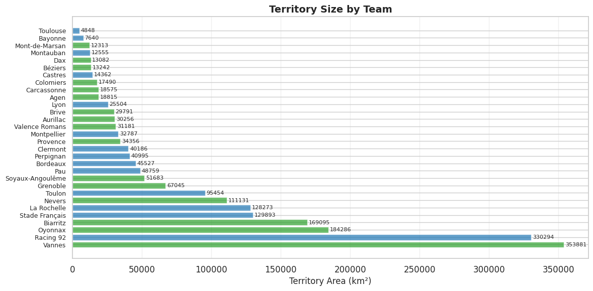
Territorial Analysis Insights:
Largest Territories: Teams in less densely populated areas or at the edges of the country tend to have larger territories. This makes sense as there are fewer neighboring teams to compete for space.
Smallest Territories: Teams in regions with multiple nearby clubs (like the southwest) have smaller, more compact territories. This reflects the competitive rugby landscape in traditional rugby regions.
League Distribution: The analysis shows how Top 14 and Pro D2 teams are distributed geographically, with some interesting patterns in territorial dominance.
Geographic Patterns#
Let’s examine the spatial distribution more closely by looking at team density in different regions of France.
# Analyze regional clustering
# Group teams by approximate regions
def assign_region(city):
    """Assign city to approximate French region"""
    city_lower = city.lower()
    if 'toulouse' in city_lower or 'castres' in city_lower or 'montpellier' in city_lower:
        return 'Occitanie'
    elif 'bordeaux' in city_lower or 'la rochelle' in city_lower or 'pau' in city_lower or 'bayonne' in city_lower:
        return 'Nouvelle-Aquitaine'
    elif 'lyon' in city_lower or 'clermont' in city_lower or 'grenoble' in city_lower or 'oyonnax' in city_lower:
        return 'Auvergne-Rhône-Alpes'
    elif 'paris' in city_lower or 'nanterre' in city_lower:
        return 'Île-de-France'
    elif 'toulon' in city_lower or 'perpignan' in city_lower:
        return 'Provence-Alpes-Côte d\'Azur'
    elif 'brive' in city_lower:
        return 'Nouvelle-Aquitaine'
    else:
        return 'Other'

teams_df['Region'] = teams_df['City'].apply(assign_region)

# Count teams by region
region_counts = teams_df.groupby('Region').agg({
    'Team': 'count',
    'League': lambda x: x.value_counts().to_dict()
}).reset_index()
region_counts.columns = ['Region', 'Team_Count', 'League_Distribution']

print("Team Distribution by Region:")
print("="*60)
for _, row in region_counts.iterrows():
    print(f"\n{row['Region']}: {row['Team_Count']} teams")
    if isinstance(row['League_Distribution'], dict):
        for league, count in row['League_Distribution'].items():
            print(f"  - {league}: {count}")

# Visualize regional distribution
fig, ax = plt.subplots(figsize=(10, 6))
region_counts_sorted = region_counts.sort_values('Team_Count', ascending=True)
bars = ax.barh(region_counts_sorted['Region'], region_counts_sorted['Team_Count'],
               color='#1f77b4', alpha=0.7)
ax.set_xlabel('Number of Teams', fontsize=12)
ax.set_title('Professional Rugby Teams by Region', fontsize=14, fontweight='bold')
ax.grid(True, alpha=0.3, axis='x')

# Add value labels
for i, (idx, row) in enumerate(region_counts_sorted.iterrows()):
    ax.text(row['Team_Count'] + 0.2, i, f"{int(row['Team_Count'])}",
            va='center', fontsize=10, fontweight='bold')

plt.tight_layout()
plt.show()
Team Distribution by Region:
============================================================

Auvergne-Rhône-Alpes: 4 teams
  - Top 14: 2
  - Pro D2: 2

Nouvelle-Aquitaine: 5 teams
  - Top 14: 4
  - Pro D2: 1

Occitanie: 3 teams
  - Top 14: 3

Other: 14 teams
  - Pro D2: 13
  - Top 14: 1

Provence-Alpes-Côte d'Azur: 2 teams
  - Top 14: 2

Île-de-France: 2 teams
  - Top 14: 2
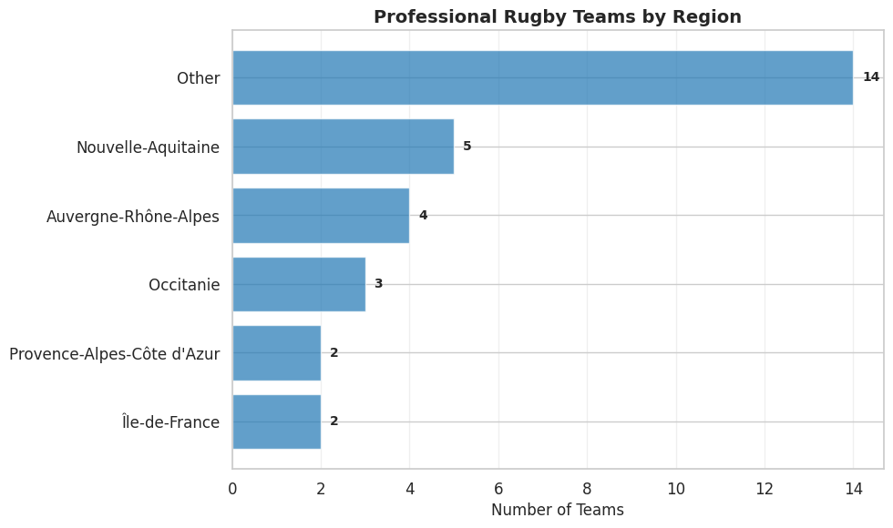
Regional Analysis Insights:
Occitanie and Nouvelle-Aquitaine Domination: These two regions in southwestern France contain the majority of professional rugby teams, confirming rugby’s traditional stronghold.
Paris Region Underrepresentation: Despite being France’s most populous region, Île-de-France has relatively few teams, leading to large territorial coverage for those teams.
Geographic Clustering: The analysis reveals clear geographic clustering, with teams concentrated in specific regions rather than evenly distributed across the country.
Conclusions#
This Voronoi analysis of French professional rugby teams reveals several important geographic patterns:
Key Findings#
Territorial Concentration: Rugby teams are heavily concentrated in southwestern France, particularly in Occitanie and Nouvelle-Aquitaine regions. This reflects the sport’s historical and cultural roots in these areas.
Sparse Northern Coverage: Northern France, despite having large population centers, has relatively few professional rugby teams. This creates large territorial regions for teams like Racing 92 and Stade Français.
Territorial Size Variation: There is significant variation in territory sizes, with some teams controlling vast regions while others have compact territories in densely populated rugby regions.
Geographic Clustering: The Voronoi diagram clearly shows clustering of teams in traditional rugby heartlands, with clear boundaries between team territories.
Implications#
Fan Base Distribution: Teams in the southwest may have more concentrated, local fan bases, while northern teams may need to draw from larger geographic areas.
Competition Intensity: Regions with multiple teams (like the southwest) show more competitive territorial boundaries, potentially reflecting stronger local rugby cultures.
Growth Opportunities: The large territories in northern France suggest potential for expansion or new team locations in underserved regions.
Technical Achievements#
This project demonstrates:
Geospatial Analysis: Application of computational geometry (Voronoi tessellation) to real-world geographic data
Data Visualization: Creation of both static and interactive maps for different use cases
Sports Analytics: Use of spatial analysis to understand sports team distribution and territorial dynamics
Future Enhancements#
Potential extensions of this analysis could include:
Overlaying population density to understand territory-to-population ratios
Historical analysis of how team geography has changed over time
Comparison with other sports (football, basketball) to see if rugby’s distribution is unique
Statistical analysis of nearest neighbor distances and territorial compactness
Integration with match attendance data to validate territorial assumptions
This analysis showcases the intersection of computational geometry, geospatial analysis, and sports analytics, demonstrating how mathematical concepts can provide insights into cultural and geographic patterns.