Holt-Winters Exponential Smoothing#
Navigation: ← Previous: Simple Exponential Smoothing | Next: Fourier Analysis →
Holt’s method adds trend; Holt-Winters adds seasonality. The ETS framework unifies error, trend, and seasonal components.
from pathlib import Path
import pandas as pd
import numpy as np
import matplotlib.pyplot as plt
import warnings
warnings.filterwarnings('ignore')
plt.style.use('seaborn-v0_8-whitegrid')

DATA_DIR = Path('data')
if not DATA_DIR.exists():
    DATA_DIR = Path('projects/time-series-analysis/data')

def load_series(name):
    """Load a bundled CSV as a DatetimeIndex Series."""
    df = pd.read_csv(DATA_DIR / name, parse_dates=['date'])
    return df.set_index('date')['value'].sort_index()

def load_air_passengers():
    path = DATA_DIR / 'air_passengers.csv'
    if path.exists():
        return load_series('air_passengers.csv')
    from statsmodels.datasets import get_rdataset
    air = get_rdataset('AirPassengers', 'datasets').data
    s = air['value']
    s.index = pd.date_range('1949-01', periods=len(s), freq='MS')
    return s

def load_milk():
    path = DATA_DIR / 'monthly_milk.csv'
    if path.exists():
        return load_series('monthly_milk.csv')
    url = 'https://raw.githubusercontent.com/jbrownlee/Datasets/master/monthly-milk-production-pounds.csv'
    return pd.read_csv(url, index_col=0, parse_dates=True).squeeze()

def load_co2():
    from statsmodels.datasets import co2
    return co2.load().data.resample('MS').mean().ffill().squeeze()

def load_sunspots():
    from statsmodels.datasets import sunspots
    d = sunspots.load_pandas().data
    return d.set_index('YEAR')['SUNACTIVITY']

def load_retail():
    path = DATA_DIR / 'uk_retail_sales.csv'
    if path.exists():
        return load_series('uk_retail_sales.csv')
    raise FileNotFoundError('uk_retail_sales.csv not found in data/')
from statsmodels.tsa.holtwinters import ExponentialSmoothing
Holt-Winters Recurrences#
Level: \(\ell_t = \alpha(y_t - s_{t-m}) + (1-\alpha)(\ell_{t-1} + b_{t-1})\)
Trend: \(b_t = \beta^*(\ell_t - \ell_{t-1}) + (1-\beta^*)b_{t-1}\)
Seasonal: \(s_t = \gamma(y_t - \ell_{t-1} - b_{t-1}) + (1-\gamma)s_{t-m}\)
Forecast: \(\hat{y}_{t+h|t} = \ell_t + hb_t + s_{t+h-m(k+1)}\)
air = load_air_passengers()
milk = load_milk()

# Multiplicative HW for Air Passengers
hw_mul = ExponentialSmoothing(
    air, trend='add', seasonal='mul', seasonal_periods=12,
    initialization_method='estimated'
).fit(optimized=True)
print(f'Air Passengers HW (mul): AIC={hw_mul.aic:.1f}')

# Additive HW for Milk
hw_add = ExponentialSmoothing(
    milk, trend='add', seasonal='add', seasonal_periods=12,
    initialization_method='estimated'
).fit(optimized=True)
print(f'Milk HW (add): AIC={hw_add.aic:.1f}')
Air Passengers HW (mul): AIC=709.9
Milk HW (add): AIC=557.3
/opt/hostedtoolcache/Python/3.11.16/x64/lib/python3.11/site-packages/statsmodels/tsa/base/tsa_model.py:480: ValueWarning: No frequency information was provided, so inferred frequency MS will be used.
  self._init_dates(dates, freq)
/opt/hostedtoolcache/Python/3.11.16/x64/lib/python3.11/site-packages/statsmodels/tsa/base/tsa_model.py:480: ValueWarning: No frequency information was provided, so inferred frequency MS will be used.
  self._init_dates(dates, freq)
# ETS model selection via AIC
configs = [
    ('SES', dict()),
    ('Holt', dict(trend='add')),
    ('HW add', dict(trend='add', seasonal='add', seasonal_periods=12)),
    ('HW mul', dict(trend='add', seasonal='mul', seasonal_periods=12)),
]
rows = []
for label, kw in configs:
    m = ExponentialSmoothing(air, initialization_method='estimated', **kw).fit(optimized=True)
    rows.append({'Model': label, 'AIC': m.aic, 'BIC': m.bic})
pd.DataFrame(rows).sort_values('AIC')
/opt/hostedtoolcache/Python/3.11.16/x64/lib/python3.11/site-packages/statsmodels/tsa/base/tsa_model.py:480: ValueWarning: No frequency information was provided, so inferred frequency MS will be used.
  self._init_dates(dates, freq)
/opt/hostedtoolcache/Python/3.11.16/x64/lib/python3.11/site-packages/statsmodels/tsa/base/tsa_model.py:480: ValueWarning: No frequency information was provided, so inferred frequency MS will be used.
  self._init_dates(dates, freq)
/opt/hostedtoolcache/Python/3.11.16/x64/lib/python3.11/site-packages/statsmodels/tsa/base/tsa_model.py:480: ValueWarning: No frequency information was provided, so inferred frequency MS will be used.
  self._init_dates(dates, freq)
/opt/hostedtoolcache/Python/3.11.16/x64/lib/python3.11/site-packages/statsmodels/tsa/base/tsa_model.py:480: ValueWarning: No frequency information was provided, so inferred frequency MS will be used.
  self._init_dates(dates, freq)
| Model | AIC | BIC | |
|---|---|---|---|
| 3 | HW mul | 709.891719 | 757.408732 |
| 2 | HW add | 753.294168 | 800.811181 |
| 0 | SES | 1016.124823 | 1022.064450 |
| 1 | Holt | 1019.488876 | 1031.368129 |
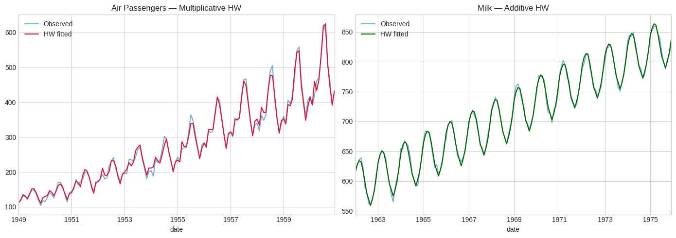
fig, axes = plt.subplots(1, 2, figsize=(14, 5))
air.plot(ax=axes[0], label='Observed', alpha=0.6)
hw_mul.fittedvalues.plot(ax=axes[0], label='HW fitted', color='crimson')
axes[0].set_title('Air Passengers — Multiplicative HW')

milk.plot(ax=axes[1], label='Observed', alpha=0.6)
hw_add.fittedvalues.plot(ax=axes[1], label='HW fitted', color='darkgreen')
axes[1].set_title('Milk — Additive HW')
for ax in axes:
    ax.legend()
fig.tight_layout()
fig
Key Takeaways#
Multiplicative vs additive: Use multiplicative when seasonal amplitude scales with level (Air Passengers).
ETS framework: All HW variants are special cases of Error-Trend-Seasonal state-space models.
Damped trend: Undamped linear trends produce unrealistic long-horizon forecasts — damped variants preferred in production.
AIC selection: Compare ETS variants systematically rather than guessing seasonal form.
Navigation: ← Previous: Simple Exponential Smoothing | Next: Fourier Analysis →