Introduction#
This chapter sets the context for a UK replication of the French systèmes urbains régionaux cartogram (Géographie-cités / DATAR, 2011). We compare the original map with a schematic of our pipeline—from TTWA nodes and census flows to Nystuen–Dacey dominant-flow partitions and a final styled cartogram.
Previous: Project overview
Next: Data acquisition
suppressPackageStartupMessages({
  library(ggplot2)
  library(patchwork)
  library(ggraph)
  library(tidygraph)
  library(igraph)
  library(here)
  library(tibble)
  library(png)
  library(grid)
})
proj_dir <- here::here("projects", "uk-urban-systems-network")
data_dir <- file.path(proj_dir, "data")
fig_dir <- file.path(proj_dir, "figures")
dir.create(data_dir, recursive = TRUE, showWarnings = FALSE)
dir.create(fig_dir, recursive = TRUE, showWarnings = FALSE)
French inspiration and UK pipeline#
french_ref <- here::here(
  "_static", "uk-urban-systems-network", "french_datar_2011.png"
)

if (!file.exists(french_ref)) {
  stop(
    "Place french_datar_2011.png in _static/uk-urban-systems-network/ ",
    "(see _static/uk-urban-systems-network/README.md)."
  )
}

# Panel A: French reference cartogram
p_french <- ggplot() +
  annotation_custom(
    rasterGrob(png::readPNG(french_ref), interpolate = TRUE),
    xmin = -Inf, xmax = Inf, ymin = -Inf, ymax = Inf
  ) +
  theme_void() +
  labs(title = "France (Géographie-cités / DATAR, 2011)")
# Panel B: schematic UK pipeline (illustrative node–edge diagram)
pipeline_edges <- tibble::tibble(
  from = c("data", "data", "nodes", "edges", "edges"),
  to = c("nodes", "edges", "partition", "partition", "map")
)
pipeline_nodes <- tibble::tibble(
  name = c("data", "nodes", "edges", "partition", "map"),
  x = c(0, 1, 2, 3, 4),
  y = c(0, 1, 0, 1, 0)
)

g_pipe <- tbl_graph(nodes = pipeline_nodes, edges = pipeline_edges, directed = TRUE)

p_pipeline <- ggraph(g_pipe, layout = "linear") +
  geom_edge_link(
    arrow = arrow(length = unit(3, "mm"), ends = "last"),
    colour = "grey40"
  ) +
  geom_node_point(size = 8, colour = "#2c3e50") +
  geom_node_text(aes(label = name), colour = "white", size = 3) +
  labs(title = "UK build-up (schematic)") +
  theme_void()

p_compare <- p_french + p_pipeline + plot_layout(ncol = 2)

fig_out <- file.path(fig_dir, "01_pipeline_schematic.png")
ggsave(fig_out, p_compare, width = 12, height = 5, dpi = 300)
invisible(fig_out)
Warning message:
“Existing variables `x` and `y` overwritten by layout variables”
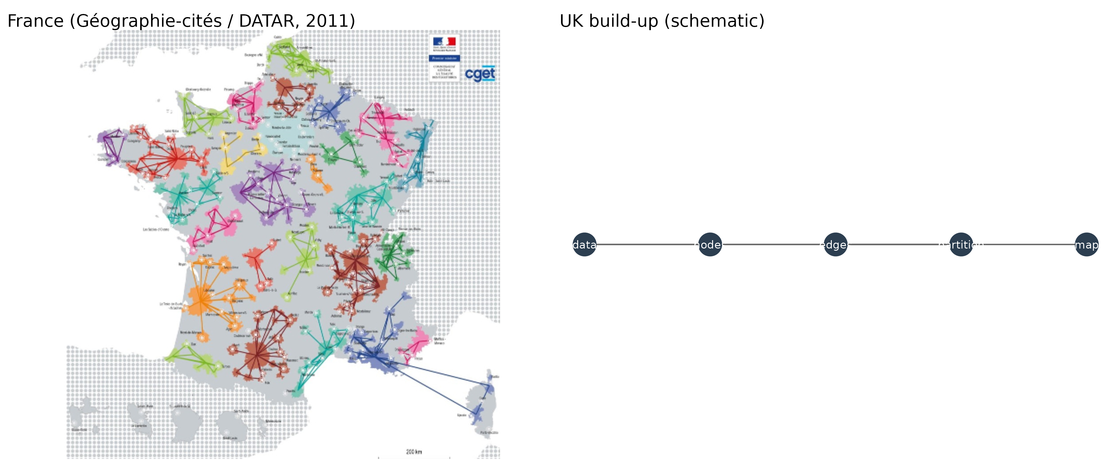
Methodology overview#
Nodes: Travel to Work Areas (TTWAs, 2011 definition) from the ONS Open Geography Portal.
Edges: Workplace-to-residence flows from the 2021 Census (NOMIS
WU03UK), aggregated to TTWA pairs.Partition: Nystuen–Dacey dominant-flow / nodal regions (Route B)—not Louvain or Infomap clustering.
Final map: Regional colours, choropleth TTWA fill, flow-weighted curved edges, and a London inset.
Data sources#
Next: Data acquisition →