Introduction & Data Loading

Navigation: ← Previous: Project Overview | Next: Simple Exponential Smoothing →

This notebook loads five benchmark time series, visualises their structure, and introduces decomposition and autocorrelation as exploratory tools. Classical methods — as opposed to modern ML forecasters — assume explicit structure (trend, seasonality, autocorrelation) that we can diagnose visually and statistically.

from pathlib import Path
import pandas as pd
import numpy as np
import matplotlib.pyplot as plt
import warnings
warnings.filterwarnings('ignore')
plt.style.use('seaborn-v0_8-whitegrid')

DATA_DIR = Path('data')
if not DATA_DIR.exists():
    DATA_DIR = Path('projects/time-series-analysis/data')

def load_series(name):
    """Load a bundled CSV as a DatetimeIndex Series."""
    df = pd.read_csv(DATA_DIR / name, parse_dates=['date'])
    return df.set_index('date')['value'].sort_index()

def load_air_passengers():
    path = DATA_DIR / 'air_passengers.csv'
    if path.exists():
        return load_series('air_passengers.csv')
    from statsmodels.datasets import get_rdataset
    air = get_rdataset('AirPassengers', 'datasets').data
    s = air['value']
    s.index = pd.date_range('1949-01', periods=len(s), freq='MS')
    return s

def load_milk():
    path = DATA_DIR / 'monthly_milk.csv'
    if path.exists():
        return load_series('monthly_milk.csv')
    url = 'https://raw.githubusercontent.com/jbrownlee/Datasets/master/monthly-milk-production-pounds.csv'
    return pd.read_csv(url, index_col=0, parse_dates=True).squeeze()

def load_co2():
    from statsmodels.datasets import co2
    return co2.load().data.resample('MS').mean().ffill().squeeze()

def load_sunspots():
    from statsmodels.datasets import sunspots
    d = sunspots.load_pandas().data
    return d.set_index('YEAR')['SUNACTIVITY']

def load_retail():
    path = DATA_DIR / 'uk_retail_sales.csv'
    if path.exists():
        return load_series('uk_retail_sales.csv')
    raise FileNotFoundError('uk_retail_sales.csv not found in data/')

Datasets

We load five canonical series covering different frequencies and features.

# Load all five benchmark datasets
air = load_air_passengers()
milk = load_milk()
co2 = load_co2()
spots = load_sunspots()
retail = load_retail()

datasets = {
    'Air Passengers': air,
    'Milk Production': milk,
    'Mauna Loa CO2': co2,
    'Sunspots': spots,
    'UK Retail Sales': retail,
}
for name, s in datasets.items():
    freq = pd.infer_freq(s.index[:3]) if isinstance(s.index, pd.DatetimeIndex) else 'annual'
    print(f"{name:20s} n={len(s):4d}  freq={freq or 'irregular'}")

Air Passengers       n= 144  freq=MS
Milk Production      n= 168  freq=MS
Mauna Loa CO2        n= 526  freq=MS
Sunspots             n= 309  freq=annual
UK Retail Sales      n= 300  freq=MS

Visualisation

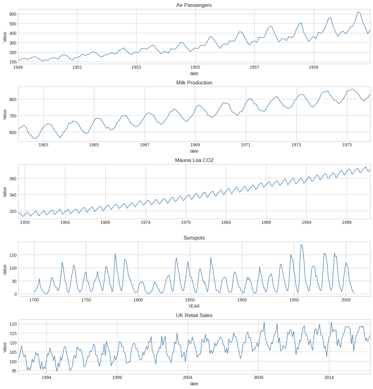
Time plots reveal trend, seasonality, and changing variance at a glance.

fig, axes = plt.subplots(len(datasets), 1, figsize=(12, 2.5 * len(datasets)), sharex=False)
for ax, (name, s) in zip(axes, datasets.items()):
    s.plot(ax=ax, color='steelblue', lw=1.2)
    ax.set_title(name)
    ax.set_ylabel('Value')
fig.tight_layout()
fig

Time Series Features

• Trend: long-run increase or decrease (Air Passengers, CO₂)

• Seasonality: fixed-period cycles (monthly period 12, annual period ~11 for sunspots)

• Cyclicality: non-fixed period oscillations

• Irregularity: noise and one-off events (UK Retail Sales)

Weak stationarity requires constant mean, constant variance, and autocovariance depending only on lag — rarely satisfied in raw economic series.

Autocorrelation

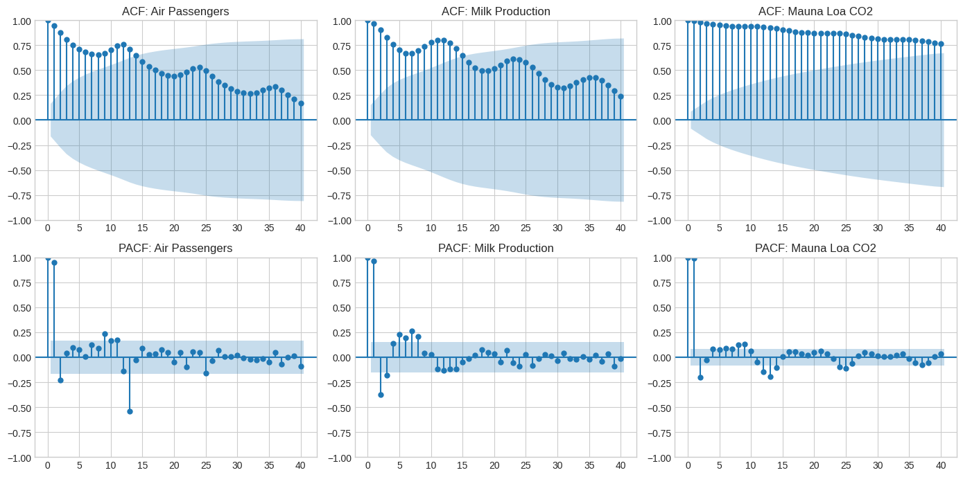
ACF and PACF summarise linear dependence at each lag.

from statsmodels.graphics.tsaplots import plot_acf, plot_pacf

fig, axes = plt.subplots(2, 3, figsize=(14, 7))
series_list = list(datasets.items())[:3]
for i, (name, s) in enumerate(series_list):
    plot_acf(s.dropna(), ax=axes[0, i], lags=min(40, len(s)//2 - 1), title=f'ACF: {name}')
    plot_pacf(s.dropna(), ax=axes[1, i], lags=min(40, len(s)//2 - 1), title=f'PACF: {name}', method='ywm')
fig.tight_layout()
fig

Classical Decomposition

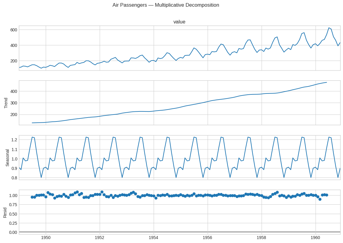
Additive: \(y_t = T_t + S_t + R_t\). Multiplicative when seasonal amplitude grows with level.

from statsmodels.tsa.seasonal import seasonal_decompose

# Air Passengers — multiplicative seasonality
decomp_mul = seasonal_decompose(air, model='multiplicative', period=12)
fig = decomp_mul.plot()
fig.set_size_inches(12, 8)
fig.suptitle('Air Passengers — Multiplicative Decomposition', y=1.02)
fig

STL Decomposition

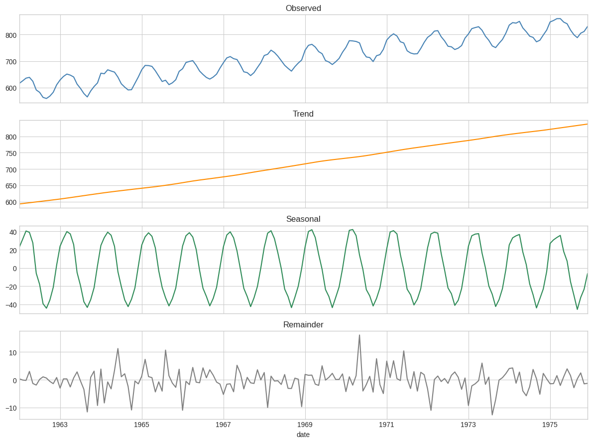
STL (Seasonal-Trend decomposition using Loess) is robust to outliers and handles evolving seasonality.

from statsmodels.tsa.seasonal import STL

stl = STL(milk, period=12, robust=True).fit()
fig, axes = plt.subplots(4, 1, figsize=(12, 9), sharex=True)
milk.plot(ax=axes[0], title='Observed', color='steelblue')
stl.trend.plot(ax=axes[1], title='Trend', color='darkorange')
stl.seasonal.plot(ax=axes[2], title='Seasonal', color='seagreen')
stl.resid.plot(ax=axes[3], title='Remainder', color='gray')
fig.tight_layout()
fig

Key Takeaways

• Benchmark diversity: Each dataset highlights different features — multiplicative season (Air Passengers), additive season (Milk), quasi-periodicity (Sunspots), trend+season (CO₂), real-world noise (Retail).

• ACF/PACF patterns: Slow decay in ACF indicates non-stationarity; spikes at lag 12 signal monthly seasonality.

• Decomposition choice: Multiplicative when seasonal swings grow with level; STL preferred when outliers or evolving season matter.

• Next steps: With features identified, we proceed to modelling — starting with the simplest forecaster, SES.

---

Navigation: ← Previous: Project Overview | Next: Simple Exponential Smoothing →