Game State Features

Navigation: ← Previous: Introduction | Next: DLS & Resource Methods →

We encode each ball in the chase as a feature vector for modelling.

import sys
from pathlib import Path
import pandas as pd
import numpy as np
import matplotlib.pyplot as plt
import warnings
warnings.filterwarnings('ignore')
plt.style.use('seaborn-v0_8-whitegrid')

PROJ_DIR = Path('.').resolve()
if not (PROJ_DIR / 'cricsheet_utils.py').exists():
    PROJ_DIR = Path('projects/cricket-win-probability').resolve()
if str(PROJ_DIR) not in sys.path:
    sys.path.insert(0, str(PROJ_DIR))

from cricsheet_utils import (
    project_data_dir, load_cricsheet_json, match_metadata, balls_to_dataframe,
    build_game_states, cumulative_runs_by_innings, resource_remaining,
    dls_win_probability,
)
DATA_DIR = project_data_dir()
SAMPLE_DIR = DATA_DIR / 'sample_matches'

training = pd.read_csv(DATA_DIR / 'odi_training_sample.csv')
feature_cols = [
    'runs_scored', 'wickets_lost', 'balls_bowled', 'balls_remaining',
    'wickets_remaining', 'runs_required', 'runs_required_per_ball',
    'current_run_rate', 'target', 'overs_completed',
    'phase_powerplay', 'phase_middle', 'phase_death',
]
training[feature_cols].describe().T

	count	mean	std	min	25%	50%	75%	max
runs_scored	120000.0	132.790708	77.812029	0.000000	66.000000	132.000000	198.000000	322.0
wickets_lost	120000.0	3.146100	2.187440	0.000000	1.000000	3.000000	5.000000	8.0
balls_bowled	120000.0	150.500000	86.602420	1.000000	75.750000	150.500000	225.250000	300.0
balls_remaining	120000.0	149.500000	86.602420	0.000000	74.750000	149.500000	224.250000	299.0
wickets_remaining	120000.0	6.853900	2.187440	2.000000	5.000000	7.000000	9.000000	10.0
runs_required	120000.0	142.649092	78.515024	0.000000	76.000000	142.000000	208.000000	341.0
runs_required_per_ball	120000.0	1.374173	5.067772	0.000000	0.862903	0.954887	1.072917	99.0
current_run_rate	120000.0	5.286491	1.054857	0.000000	4.813187	5.288136	5.740385	30.0
target	120000.0	275.375000	22.463161	220.000000	260.000000	276.000000	290.250000	341.0
overs_completed	120000.0	25.083333	14.433737	0.166667	12.625000	25.083333	37.541667	50.0
phase_powerplay	120000.0	0.200000	0.400002	0.000000	0.000000	0.000000	0.000000	1.0
phase_middle	120000.0	0.580000	0.493561	0.000000	0.000000	1.000000	1.000000	1.0
phase_death	120000.0	0.220000	0.414248	0.000000	0.000000	0.000000	0.000000	1.0

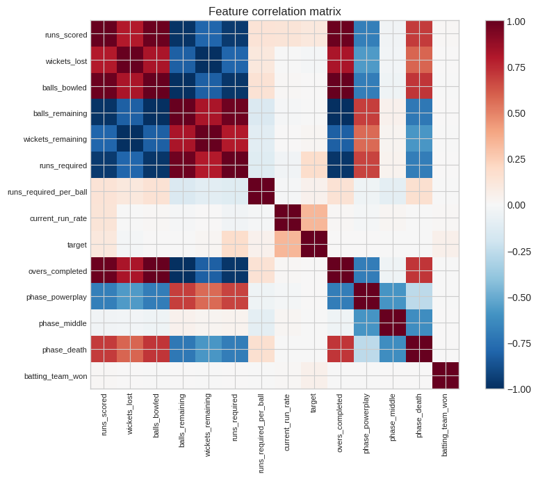
Correlation structure

corr = training[feature_cols + ['batting_team_won']].corr()
fig, ax = plt.subplots(figsize=(9, 7))
im = ax.imshow(corr, cmap='RdBu_r', vmin=-1, vmax=1)
ax.set_xticks(range(len(corr)))
ax.set_yticks(range(len(corr)))
ax.set_xticklabels(corr.columns, rotation=90, fontsize=8)
ax.set_yticklabels(corr.columns, fontsize=8)
plt.colorbar(im, ax=ax)
ax.set_title('Feature correlation matrix')
plt.tight_layout()
plt.show()

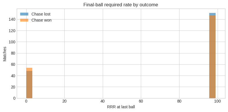
RRR vs outcome at the final ball

finals = training.groupby('match_idx').tail(1)
fig, ax = plt.subplots(figsize=(8, 4))
for won, grp in finals.groupby('batting_team_won'):
    label = 'Chase won' if won else 'Chase lost'
    ax.hist(grp['runs_required_per_ball'].dropna(), bins=30, alpha=0.6, label=label)
ax.set_xlabel('RRR at last ball')
ax.set_ylabel('Matches')
ax.legend()
ax.set_title('Final-ball required rate by outcome')
plt.tight_layout()
plt.show()

Example: high-pressure state

pressure = training[(training['over'] >= 43) & (training['wickets_lost'] >= 5)]
pressure.nlargest(1, 'runs_required_per_ball')[feature_cols + ['batting_team_won']]

	runs_scored	wickets_lost	balls_bowled	balls_remaining	wickets_remaining	runs_required	runs_required_per_ball	current_run_rate	target	overs_completed	phase_powerplay	phase_middle	phase_death	batting_team_won
299	228	6	300	0	4	6	99.0	4.56	234	50.0	0	0	1	1

---

Navigation: ← Previous: Introduction | Next: DLS & Resource Methods →