Top 14 (France)

Top 14 (France)#

The Top 14 is France’s premier professional rugby union league. This notebook samples SRTM 30 arc-second elevation from geodata::elevation_30s(country = "FRA") at each club’s usual home ground and maps the results on a cropped national terrain surface.

Stadium coordinates below use approximate centre points for each club’s usual home ground. La Rochelle (Stade Marcel-Deflandre / Stade Rochelais) uses the published WGS84 location (46.158°N, 1.178°W). Replace the top14_clubs table and rebuild if you need a different season’s venues or survey-grade coordinates.

top14_clubs <- data.frame(
  club = c(
    "Toulouse", "Toulon", "La Rochelle", "Bordeaux", "Racing 92",
    "Stade Français", "Clermont", "Lyon", "Castres", "Montpellier",
    "Bayonne", "Pau", "Perpignan", "Montauban"
  ),
  stadium = c(
    "Stade Ernest-Wallon", "Stade Mayol", "Stade Marcel-Deflandre (Stade Rochelais)",
    "Matmut Atlantique", "Paris La Défense Arena", "Stade Jean-Bouin",
    "Stade Marcel-Michelin", "Matmut Stadium Gerland", "Stade Pierre-Fabre",
    "GGL Stadium", "Stade Jean-Dauger", "Stade du Hameau",
    "Stade Aimé-Giral", "Stade Sapiac"
  ),
  city = c(
    "Toulouse", "Toulon", "La Rochelle", "Bordeaux", "Nanterre",
    "Paris", "Clermont-Ferrand", "Lyon", "Castres", "Montpellier",
    "Bayonne", "Pau", "Perpignan", "Montauban"
  ),
  lon = c(
    1.415, 5.934, -1.17806, -0.598, 2.229,
    2.252, 3.106, 4.832, 2.249, 3.861,
    -1.486, -0.322, 2.894, 1.355
  ),
  lat = c(
    43.621, 43.125, 46.15806, 44.829, 48.895,
    48.844, 45.791, 45.724, 43.601, 43.590,
    43.484, 43.303, 42.711, 44.017
  ),
  region = c(
    "Occitanie", "Provence", "Atlantic coast", "Nouvelle-Aquitaine", "Paris",
    "Paris", "Massif Central", "Rhône-Alpes", "Occitanie", "Occitanie",
    "Basque Country", "Pyrenees", "Occitanie", "Occitanie"
  ),
  stringsAsFactors = FALSE
)

top14_sv <- terra::vect(top14_clubs, geom = c("lon", "lat"), crs = "EPSG:4326")

Download elevation (France)#

fra_elev <- geodata::elevation_30s(country = "FRA", path = tempdir())
fra_boundary <- rnaturalearth::ne_countries(
  country = "France",
  scale = "medium",
  returnclass = "sv"
)

if (!terra::same.crs(fra_elev, fra_boundary)) {
  fra_boundary <- terra::project(fra_boundary, fra_elev)
}

fra_elev_masked <- terra::mask(terra::crop(fra_elev, fra_boundary), fra_boundary)
elev_layer <- names(fra_elev_masked)[1]
fra_elev_masked <- fra_elev_masked |>
  tidyterra::rename(elevation = !!rlang::sym(elev_layer))

Cached as: /tmp/Rtmp5W238T/elevation/FRA_elv_msk.zip

Extract elevation per ground#

Coastal grounds can fall on SRTM water cells (NA) when the 30 arc-second grid classifies harbour or tidal flats as offshore. For any NA at a stadium point we take the nearest land cell on the cropped (unmasked) national tile so the value still reflects local relief.

extract_ground_elev <- function(r, lon, lat, radius_deg = 0.05) {
  val <- terra::extract(r, cbind(lon, lat))[[1]]
  if (!is.na(val)) {
    return(as.numeric(val))
  }
  bb <- terra::ext(
    lon - radius_deg,
    lon + radius_deg,
    lat - radius_deg,
    lat + radius_deg
  )
  sub <- terra::crop(r, bb)
  cells <- which(!is.na(terra::values(sub)))
  if (!length(cells)) {
    return(NA_real_)
  }
  xy <- terra::xyFromCell(sub, cells)
  dist2 <- (xy[, 1] - lon)^2 + (xy[, 2] - lat)^2
  vals <- terra::values(sub)[cells]
  as.numeric(vals[which.min(dist2)])
}

fra_elev_crop <- terra::crop(fra_elev, fra_boundary)
names(fra_elev_crop) <- "elevation"

top14_elev <- top14_clubs |>
  mutate(
    ground_elevation_m = mapply(
      extract_ground_elev,
      lon,
      lat,
      MoreArgs = list(r = fra_elev_crop),
      USE.NAMES = FALSE
    )
  )

top14_elev |>
  arrange(desc(ground_elevation_m)) |>
  knitr::kable(
    digits = 1,
    caption = "Top 14 grounds ranked by extracted elevation (m a.s.l.; FRA SRTM tile)"
  )

Table: Top 14 grounds ranked by extracted elevation (m a.s.l.; FRA SRTM tile)

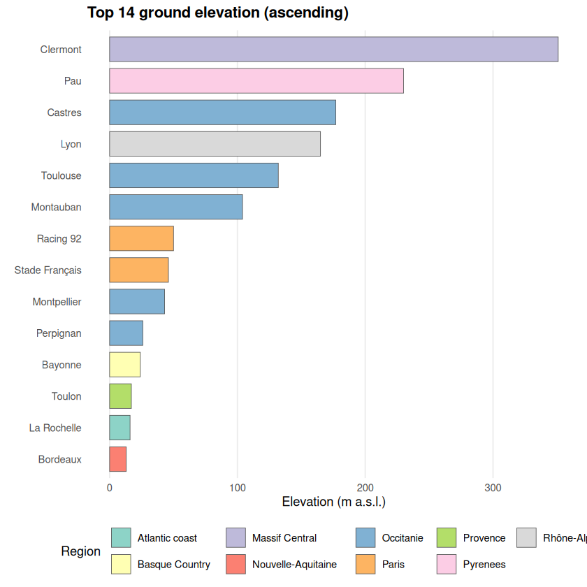
|club           |stadium                                  |city             |  lon|  lat|region             | ground_elevation_m|
|:--------------|:----------------------------------------|:----------------|----:|----:|:------------------|------------------:|
|Clermont       |Stade Marcel-Michelin                    |Clermont-Ferrand |  3.1| 45.8|Massif Central     |                351|
|Pau            |Stade du Hameau                          |Pau              | -0.3| 43.3|Pyrenees           |                230|
|Castres        |Stade Pierre-Fabre                       |Castres          |  2.2| 43.6|Occitanie          |                177|
|Lyon           |Matmut Stadium Gerland                   |Lyon             |  4.8| 45.7|Rhône-Alpes        |                165|
|Toulouse       |Stade Ernest-Wallon                      |Toulouse         |  1.4| 43.6|Occitanie          |                132|
|Montauban      |Stade Sapiac                             |Montauban        |  1.4| 44.0|Occitanie          |                104|
|Racing 92      |Paris La Défense Arena                   |Nanterre         |  2.2| 48.9|Paris              |                 50|
|Stade Français |Stade Jean-Bouin                         |Paris            |  2.3| 48.8|Paris              |                 46|
|Montpellier    |GGL Stadium                              |Montpellier      |  3.9| 43.6|Occitanie          |                 43|
|Perpignan      |Stade Aimé-Giral                         |Perpignan        |  2.9| 42.7|Occitanie          |                 26|
|Bayonne        |Stade Jean-Dauger                        |Bayonne          | -1.5| 43.5|Basque Country     |                 24|
|Toulon         |Stade Mayol                              |Toulon           |  5.9| 43.1|Provence           |                 17|
|La Rochelle    |Stade Marcel-Deflandre (Stade Rochelais) |La Rochelle      | -1.2| 46.2|Atlantic coast     |                 16|
|Bordeaux       |Matmut Atlantique                        |Bordeaux         | -0.6| 44.8|Nouvelle-Aquitaine |                 13|

Clermont and Pau sit on the Massif Central and Pyrenean foothills, where the 30 arc-second DEM routinely returns the highest values in this league. Paris clubs (Racing 92, Stade Français) and La Rochelle on the Atlantic coast tend to rank lower (at La Rochelle the stadium grid cell is classified as water in SRTM, so we report elevation from the nearest land cell a few hundred metres inland). Toulon and Perpignan are coastal but the grid cells can still reflect nearby relief.

top14_bar <- top14_elev |>
  mutate(club = stats::reorder(club, ground_elevation_m))

ggplot(top14_bar, aes(x = club, y = ground_elevation_m, fill = region)) +
  geom_col(width = 0.78, colour = "grey35", linewidth = 0.25) +
  coord_flip() +
  scale_fill_brewer(palette = "Set3", name = "Region") +
  labs(
    title = "Top 14 ground elevation (ascending)",
    x = NULL,
    y = "Elevation (m a.s.l.)"
  ) +
  theme_minimal(base_size = 11) +
  theme(
    plot.title = element_text(face = "bold", hjust = 0, margin = margin(b = 8)),
    panel.grid.major.y = element_blank(),
    panel.grid.minor = element_blank(),
    legend.position = "bottom"
  )

../../_images/b50f059587862434c17553f83994ebda00e27006c8fc7a65dba786b7d73793fe.png

Map (France)#

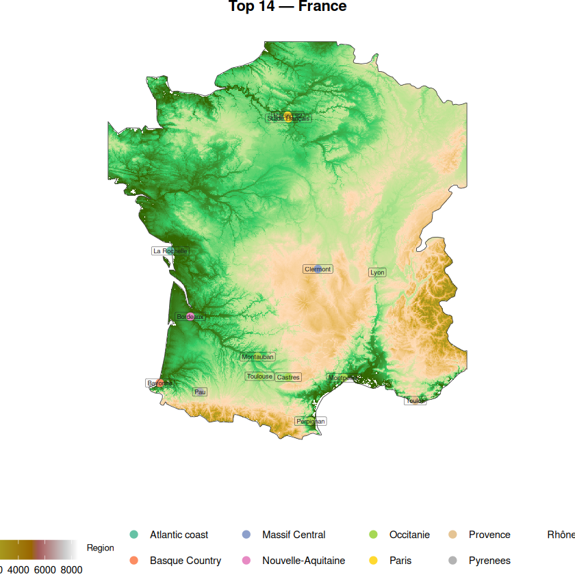
We crop the national raster to a modest bounding box around the Top 14 grounds so the map aspect remains readable.

map_ext <- terra::extend(terra::ext(top14_sv), 1.5)
r_top14 <- terra::crop(fra_elev_masked, map_ext)
outline_top14 <- terra::crop(fra_boundary, map_ext)

if (!terra::same.crs(r_top14, outline_top14)) {
  outline_top14 <- terra::project(outline_top14, r_top14)
}

ggplot() +
  tidyterra::geom_spatraster(data = r_top14, aes(fill = elevation)) +
  tidyterra::scale_fill_hypso_tint_c(
    name = "m",
    guide = guide_colorbar(barwidth = unit(3.5, "cm"), title.position = "top")
  ) +
  tidyterra::geom_spatvector(data = top14_sv, aes(colour = region), size = 2.8, show.legend = TRUE) +
  tidyterra::geom_spatvector_label(
    data = top14_sv,
    aes(label = club),
    size = 2,
    colour = "grey10",
    label.size = 0.12,
    show.legend = FALSE
  ) +
  tidyterra::geom_spatvector(data = outline_top14, fill = NA, colour = "grey25", linewidth = 0.25) +
  scale_colour_brewer(palette = "Set2", name = "Region") +
  labs(title = "Top 14 — France") +
  theme_void() +
  theme(
    plot.title = element_text(face = "bold", hjust = 0.5, margin = margin(b = 4)),
    legend.title = element_text(size = 8),
    legend.position = "bottom"
  )

<SpatRaster> resampled to 500656 cells.

Warning message:
“The `label.size` argument of `geom_label()` is deprecated as of ggplot2 3.5.0.
ℹ Please use the `linewidth` argument instead.
ℹ The deprecated feature was likely used in the tidyterra package.
  Please report the issue at <https://github.com/dieghernan/tidyterra/issues>.”

Warning message in st_point_on_surface.sfc(sf::st_zm(x)):
“st_point_on_surface may not give correct results for longitude/latitude data”

Warning message in RColorBrewer::brewer.pal(n, pal):
“n too large, allowed maximum for palette Set2 is 8
Returning the palette you asked for with that many colors
”

Warning message:
“Removed 1 row containing missing values or values outside the scale range
(`geom_sf()`).”

../../_images/db6f13e500f2170a3a1a2891b3805745b5b77f9a235f9528819f0729ac268b9e.png

Interactive map#

The map below uses Leaflet (via htmlwidgets). You can pan, zoom, and click stadium markers for club, venue, and extracted elevation. Marker colours follow the same elevation colour scale as the terrain layer. An internet connection is required for the light basemap tiles.

Top 14 — France (interactive)

The static and interactive maps highlight how France’s rugby heartland in the south-west mixes coastal venues with Massif Central and Pyrenean outliers—useful context when comparing ground elevation across the league.