library(tidyterra)
library(terra)
library(geodata)
library(rnaturalearth)
library(ggplot2)
library(dplyr)
library(sf)
library(rlang)
library(knitr)
library(leaflet)
library(htmlwidgets)
library(htmltools)
library(raster)
library(IRdisplay)

Attaching package: ‘tidyterra’

The following object is masked from ‘package:stats’:

    filter

terra 1.9.46

Attaching package: ‘dplyr’

The following objects are masked from ‘package:terra’:

    intersect, union

The following objects are masked from ‘package:stats’:

    filter, lag

The following objects are masked from ‘package:base’:

    intersect, setdiff, setequal, union

Linking to GEOS 3.12.1, GDAL 3.8.4, PROJ 9.4.0; sf_use_s2() is TRUE

Attaching package: ‘knitr’

The following object is masked from ‘package:terra’:

    spin

Loading required package: sp

Attaching package: ‘raster’

The following object is masked from ‘package:dplyr’:

    select

The following object is masked from ‘package:tidyterra’:

    select

Reloading the elevation surface

This notebook rebuilds the UK elevation raster the same way as in 01_terrain_analysis.Rmd, so it can be rendered on its own. In a larger project you might save an intermediate GeoTIFF under data/ and read it with terra::rast() to avoid duplicate downloads.

uk_elev <- geodata::elevation_30s(country = "GBR", path = tempdir())
uk_boundary <- rnaturalearth::ne_countries(
  country = "United Kingdom",
  scale = "medium",
  returnclass = "sv"
)

if (!terra::same.crs(uk_elev, uk_boundary)) {
  uk_boundary <- terra::project(uk_boundary, uk_elev)
}

uk_elev_masked <- terra::mask(terra::crop(uk_elev, uk_boundary), uk_boundary)
elev_layer <- names(uk_elev_masked)[1]
uk_elev_masked <- uk_elev_masked |>
  tidyterra::rename(elevation = !!rlang::sym(elev_layer))

Cached as: /tmp/RtmpMqMzPw/elevation/GBR_elv_msk.zip

Club locations and CRS

Premiership grounds are stored as a data frame of longitude and latitude in decimal degrees. EPSG:4326 is the standard WGS84 geographic CRS used by GPS and most global rasters (including the elevation and WorldClim grids used here): positions are angles on the ellipsoid, not metres on a flat map.

rclubs <- data.frame(
  club = c(
    "Bath Rugby", "Bristol Bears", "Exeter Chiefs", "Gloucester Rugby",
    "Harlequins", "Leicester Tigers", "Newcastle Falcons",
    "Northampton Saints", "Sale Sharks", "Saracens"
  ),
  lon = c(
    -2.361, -2.571, -3.525, -2.243, -0.215, -1.133,
    -1.622, -0.906, -2.338, -0.100
  ),
  lat = c(
    51.381, 51.455, 50.730, 51.866, 51.481, 52.620,
    54.961, 52.241, 53.419, 51.674
  ),
  region = c(
    "South West", "South West", "South West", "South West",
    "London", "Midlands", "North",
    "Midlands", "North", "London"
  )
)

clubs_sv <- terra::vect(rclubs, geom = c("lon", "lat"), crs = "EPSG:4326")

Raster–point extraction

terra::extract() performs a spatial intersection between a raster and a set of sample locations (points, polygons, or another raster). For points, each location receives the cell value(s) of the raster layer(s) at the containing cell (by default the cell centre rule applies for points). That is how we attach terrain height at each stadium to the club table.

elev_at_clubs <- terra::extract(uk_elev_masked, clubs_sv)

clubs_elev <- rclubs |>
  mutate(ground_elevation_m = elev_at_clubs[["elevation"]])

clubs_elev |>
  arrange(desc(ground_elevation_m)) |>
  kable(digits = 1, caption = "Premiership grounds ranked by extracted elevation (m)")

Table: Premiership grounds ranked by extracted elevation (m)

|club               |  lon|  lat|region     | ground_elevation_m|
|:------------------|----:|----:|:----------|------------------:|
|Leicester Tigers   | -1.1| 52.6|Midlands   |                 82|
|Northampton Saints | -0.9| 52.2|Midlands   |                 63|
|Saracens           | -0.1| 51.7|London     |                 58|
|Exeter Chiefs      | -3.5| 50.7|South West |                 50|
|Bath Rugby         | -2.4| 51.4|South West |                 31|
|Newcastle Falcons  | -1.6| 55.0|North      |                 29|
|Sale Sharks        | -2.3| 53.4|North      |                 28|
|Gloucester Rugby   | -2.2| 51.9|South West |                 18|
|Bristol Bears      | -2.6| 51.5|South West |                 14|
|Harlequins         | -0.2| 51.5|London     |                  8|

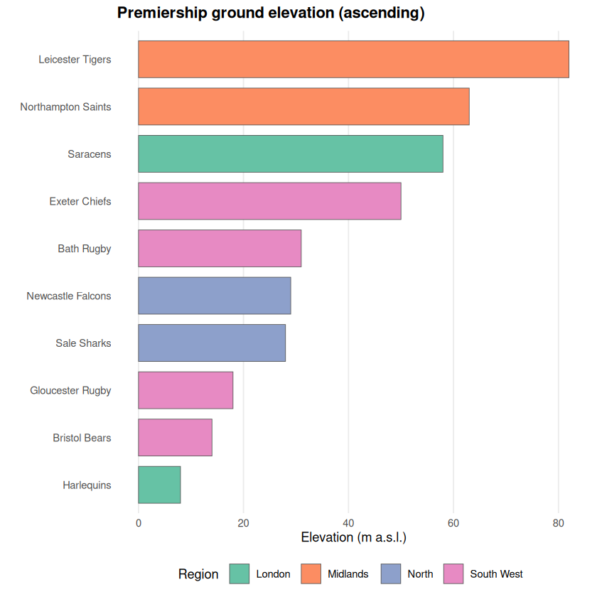
Geographically, south-western clubs such as Exeter Chiefs sit on higher ground than London sides (Harlequins, Saracens), which lie in the low-lying Thames basin. Newcastle Falcons in the north-east can be relatively high or low depending on fine-scale coastal versus inland cells, but the table makes the ranking explicit from the grid we used.

The bar chart below uses the same extracted elevations, with clubs ordered from lowest to highest ground so you can read off the full spread at a glance (still tied to the SRTM-scale raster cells used above).

clubs_elev_bar <- clubs_elev |>
  mutate(club = stats::reorder(club, ground_elevation_m))

ggplot(clubs_elev_bar, aes(x = club, y = ground_elevation_m, fill = region)) +
  geom_col(width = 0.78, colour = "grey35", linewidth = 0.25) +
  coord_flip() +
  scale_fill_brewer(palette = "Set2", name = "Region") +
  labs(
    title = "Premiership ground elevation (ascending)",
    x = NULL,
    y = "Elevation (m a.s.l.)"
  ) +
  theme_minimal(base_size = 11) +
  theme(
    plot.title = element_text(face = "bold", hjust = 0, margin = margin(b = 8)),
    panel.grid.major.y = element_blank(),
    panel.grid.minor = element_blank(),
    legend.position = "bottom"
  )

ggplot() +
  tidyterra::geom_spatraster(data = uk_elev_masked, aes(fill = elevation)) +
  tidyterra::scale_fill_hypso_tint_c(
    name = "m a.s.l.",
    guide = guide_colorbar(barwidth = unit(3.5, "cm"), title.position = "top")
  ) +
  tidyterra::geom_spatvector(data = clubs_sv, aes(colour = region), size = 3, show.legend = TRUE) +
  tidyterra::geom_spatvector_label(
    data = clubs_sv,
    aes(label = club),
    size = 2.4,
    colour = "grey10",
    label.size = 0.15,
    show.legend = FALSE
  ) +
  tidyterra::geom_spatvector(data = uk_boundary, fill = NA, colour = "grey15", linewidth = 0.3) +
  scale_colour_brewer(palette = "Set2", name = "Region") +
  labs(title = "English Premiership Rugby Grounds by Elevation") +
  theme_void() +
  theme(
    plot.title = element_text(hjust = 0.5, face = "bold", margin = margin(b = 6)),
    legend.title = element_text(size = 9),
    legend.position = "bottom"
  )

<SpatRaster> resampled to 500980 cells.

Warning message:
“The `label.size` argument of `geom_label()` is deprecated as of ggplot2 3.5.0.
ℹ Please use the `linewidth` argument instead.
ℹ The deprecated feature was likely used in the tidyterra package.
  Please report the issue at <https://github.com/dieghernan/tidyterra/issues>.”

Warning message in st_point_on_surface.sfc(sf::st_zm(x)):
“st_point_on_surface may not give correct results for longitude/latitude data”

Interactive map

The map below uses Leaflet (via htmlwidgets). You can pan, zoom, and click stadium markers for club, region, and extracted elevation. Marker colours follow the same elevation colour scale as the terrain layer. An internet connection is required for the light basemap tiles.

English Premiership (interactive)

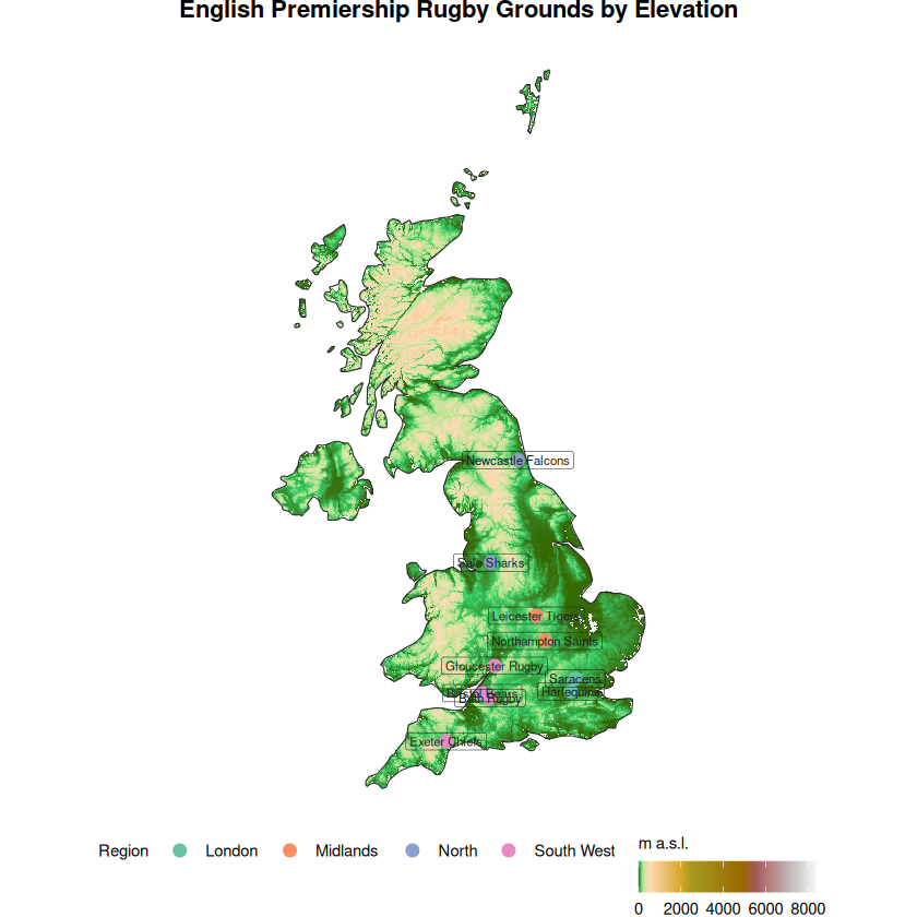
geom_spatvector_label() draws text from SpatVector attributes; where labels crowd together in static output, ggrepel could be swapped in with an sf conversion for automatic jittering.