Interpretation

Navigation: ← Previous: Deep Learning | Next: Evaluation →

What each model uses: inverse-mapped logistic weights, grouped forest importances, and Grad-CAM overlays.

Three kinds of explanation

1. Linear map. Logistic coefficients in PCA space, mapped back to 128×128 pixels (undoing PCA and standardisation). Red regions raise the malignant logit.

2. Feature families. Random-forest Gini importance plus grouped permutation (shuffle all HOG bins together, then LBP, then intensity) measured as drop in ROC-AUC.

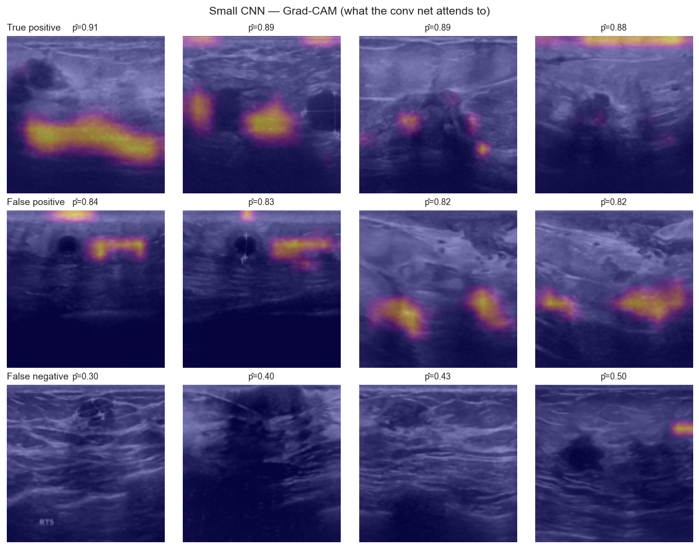
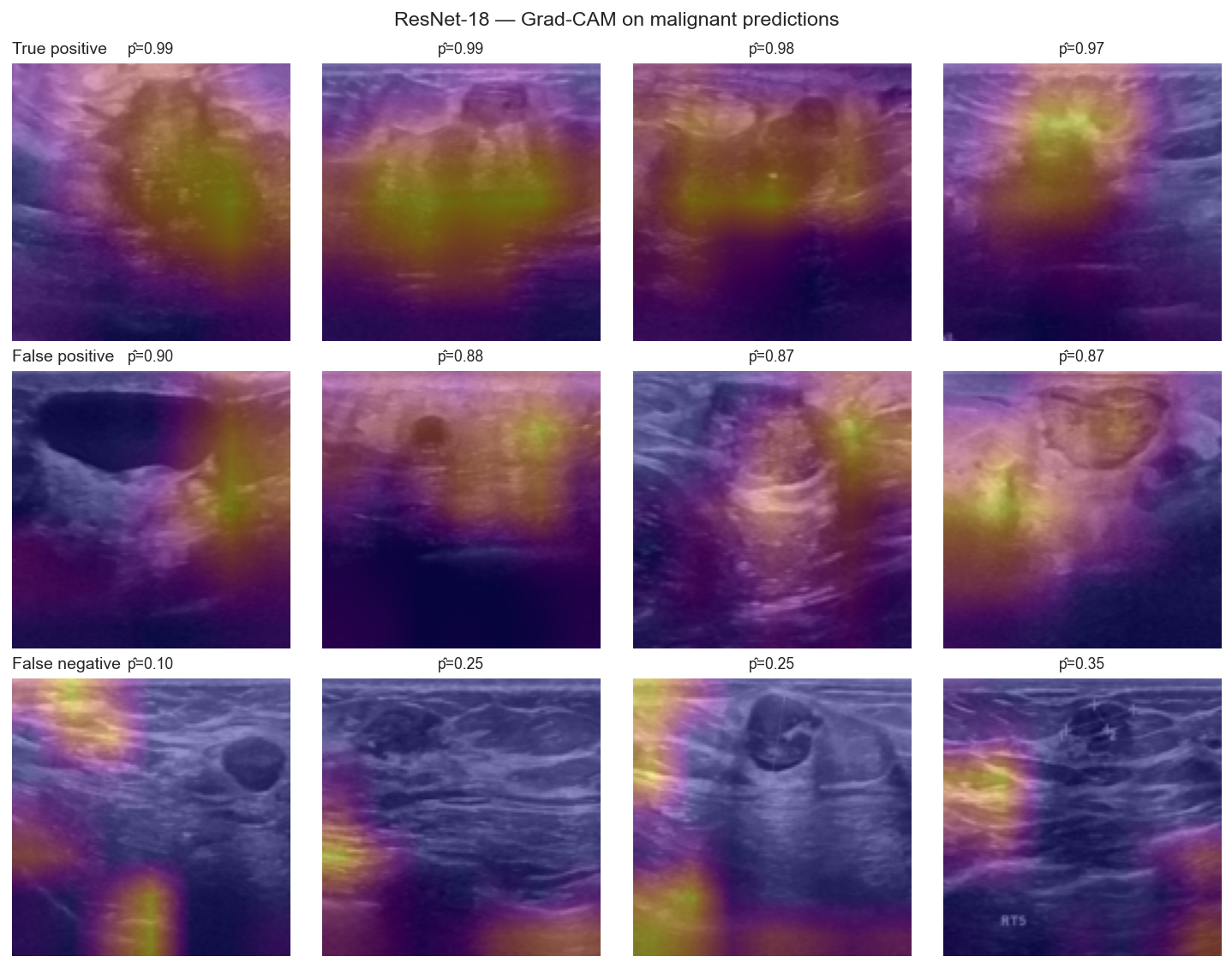
3. Grad-CAM. For each conv net, the last convolutional feature map is weighted by the gradient of the malignant logit. Overlays are shown for true positives, false positives, and false negatives on the test set.

import sys
from pathlib import Path
import numpy as np
import pandas as pd
import matplotlib.pyplot as plt
import warnings
warnings.filterwarnings("ignore")
plt.style.use("seaborn-v0_8-whitegrid")

PROJ_DIR = Path(".").resolve()
if not (PROJ_DIR / "cancer_cv_utils.py").exists():
    PROJ_DIR = Path("projects/cancer-imaging").resolve()
if str(PROJ_DIR) not in sys.path:
    sys.path.insert(0, str(PROJ_DIR))

from cancer_cv_utils import (
    CLASS_NAMES,
    METRIC_ORDER,
    artifacts_dir,
    classification_metrics,
    display_plotly,
    extract_cv_features,
    figures_dir,
    grouped_importance,
    load_metrics,
    load_predictions,
    load_splits,
    metrics_frame,
    overlay_heatmap,
    tune_threshold,
)

SPLITS = load_splits()
FIG = figures_dir()
ART = artifacts_dir()
print("Splits:", {k: v["labels"].shape[0] for k, v in SPLITS.items()})
print("Malignant rates:", {k: f"{v['labels'].mean():.1%}" for k, v in SPLITS.items()})

Splits: {'train': 546, 'val': 78, 'test': 156}
Malignant rates: {'train': '26.9%', 'val': '26.9%', 'test': '26.9%'}

from IPython.display import Image, display

Logistic regression — which pixels?

display(Image(str(FIG / '04_logistic_coef.png')))

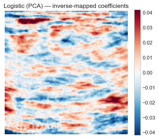
The map is a global explanation: one weight image for the whole test set, not a per-case heatmap. Because PCA mixes pixels, the pattern is spatially smooth rather than a sharp lesion outline. Treat it as ‘where a linear model can put weight’, not as a segmentation.

Random forest — which feature family?

imp = pd.read_csv(ART / 'rf_grouped_importance.csv')
display(imp.round(3))
display(Image(str(FIG / '04_rf_groups.png')))

	group	importance	permutation_auc
0	HOG (oriented edges)	0.982	0.381
1	LBP (local texture)	0.009	0.001
2	Intensity / darkness	0.009	0.002

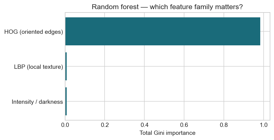
HOG (oriented edges) dominates both Gini share and the permutation drop in AUC. That matches the radiology story: margins and shadowing are edge structure. LBP texture and raw intensity add little once HOG is present — the forest is mostly an edge detector with a non-linear head.

Small CNN — Grad-CAM

display(Image(str(FIG / '04_gradcam_cnn.png')))

ResNet-18 — Grad-CAM

display(Image(str(FIG / '04_gradcam_resnet.png')))

How to read the grids

• True positives with high \(\hat p\) should light up the mass or its posterior shadow, not the empty periphery.

• False positives show the shortcuts: a benign cyst, a bright artefact, or a measurement crosshair that happens to correlate with labels.

• False negatives are the dangerous misses. If Grad-CAM ignores a visible irregular mass, the representation failed; if the mass is subtle even to the eye at 128×128, the limit is the data.

Grad-CAM is a localisation hint, not a proof of causal reasoning. It cannot tell us the model understands malignancy — only where in the pixel grid the malignant logit is sensitive.

---

Navigation: ← Previous: Deep Learning | Next: Evaluation →