Classical Models#
Navigation: ← Previous: Images & Labels | Next: Deep Learning →
A majority dummy, logistic regression on PCA-reduced pixels, and a random forest on HOG / LBP / intensity features.
Why start simple?#
With 546 training images, a model that sees 16,384 raw pixels is over-parameterised. The first two models force a strong inductive bias: (1) a linear decision in a 20–80 dimensional PCA subspace, and (2) engineered edge/texture descriptors that computer vision used for a decade before conv nets. Both train in seconds and give a yardstick the CNNs have to beat.
All reported numbers in this chapter are test-set scores. PCA rank and the forest’s decision threshold are chosen on the validation split only.
import sys
from pathlib import Path
import numpy as np
import pandas as pd
import matplotlib.pyplot as plt
import warnings
warnings.filterwarnings("ignore")
plt.style.use("seaborn-v0_8-whitegrid")

PROJ_DIR = Path(".").resolve()
if not (PROJ_DIR / "cancer_cv_utils.py").exists():
    PROJ_DIR = Path("projects/cancer-imaging").resolve()
if str(PROJ_DIR) not in sys.path:
    sys.path.insert(0, str(PROJ_DIR))

from cancer_cv_utils import (
    CLASS_NAMES,
    METRIC_ORDER,
    artifacts_dir,
    classification_metrics,
    display_plotly,
    extract_cv_features,
    figures_dir,
    grouped_importance,
    load_metrics,
    load_predictions,
    load_splits,
    metrics_frame,
    overlay_heatmap,
    tune_threshold,
)

SPLITS = load_splits()
FIG = figures_dir()
ART = artifacts_dir()
print("Splits:", {k: v["labels"].shape[0] for k, v in SPLITS.items()})
print("Malignant rates:", {k: f"{v['labels'].mean():.1%}" for k, v in SPLITS.items()})
Splits: {'train': 546, 'val': 78, 'test': 156}
Malignant rates: {'train': '26.9%', 'val': '26.9%', 'test': '26.9%'}
Dummy classifier#
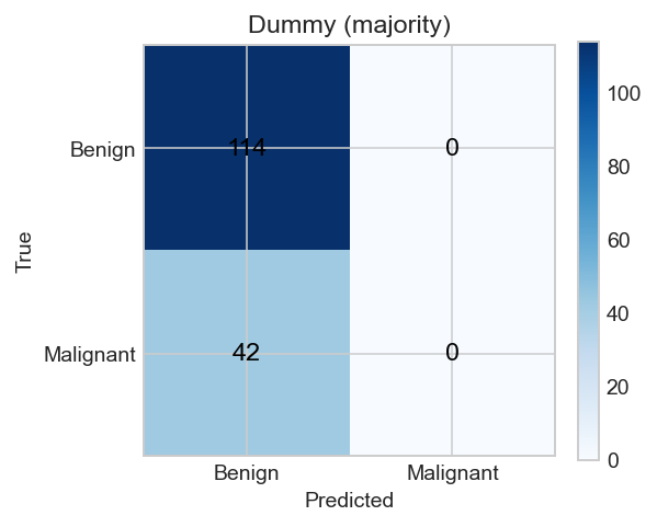
Always predict the majority class (benign / normal). Accuracy looks respectable; cancer detection is zero.
from sklearn.dummy import DummyClassifier
from IPython.display import Image, display

y_tr, y_te = SPLITS['train']['labels'], SPLITS['test']['labels']
x_tr = SPLITS['train']['images'].reshape(len(y_tr), -1)
x_te = SPLITS['test']['images'].reshape(len(y_te), -1)
dummy = DummyClassifier(strategy='most_frequent', random_state=42).fit(x_tr, y_tr)
dummy_prob = dummy.predict_proba(x_te)[:, 1]
dummy_mets = classification_metrics(y_te, dummy_prob)
pd.Series(dummy_mets)[METRIC_ORDER].to_frame('Dummy (majority)')
| Dummy (majority) | |
|---|---|
| accuracy | 0.730769 |
| precision | 0.000000 |
| recall | 0.000000 |
| f1 | 0.000000 |
| specificity | 1.000000 |
| balanced_accuracy | 0.500000 |
| roc_auc | 0.500000 |
| pr_auc | 0.269231 |
| brier | 0.269231 |
| mcc | 0.000000 |
Logistic regression on PCA-reduced pixels#
Each image is flattened, standardised, and projected to \(k\) principal components. \(k\) is picked by validation ROC-AUC from \(\{20,40,60,80\}\). Class-weighted logistic regression then predicts malignancy. The decision threshold is tuned on validation F1 so we are not locked to 0.5 on a 27% positive class.
from sklearn.decomposition import PCA
from sklearn.linear_model import LogisticRegression
from sklearn.pipeline import Pipeline
from sklearn.preprocessing import StandardScaler

x_va = SPLITS['val']['images'].reshape(len(SPLITS['val']['labels']), -1)
y_va = SPLITS['val']['labels']
best_auc, best_k = -1, 40
for k in (20, 40, 60, 80):
    pipe = Pipeline([
        ('scaler', StandardScaler()),
        ('pca', PCA(n_components=k, random_state=42)),
        ('clf', LogisticRegression(max_iter=1000, class_weight='balanced', random_state=42)),
    ]).fit(x_tr, y_tr)
    auc = classification_metrics(y_va, pipe.predict_proba(x_va)[:, 1])['roc_auc']
    if auc > best_auc:
        best_auc, best_k = auc, k

logreg = Pipeline([
    ('scaler', StandardScaler()),
    ('pca', PCA(n_components=best_k, random_state=42)),
    ('clf', LogisticRegression(max_iter=1000, class_weight='balanced', random_state=42)),
]).fit(x_tr, y_tr)
log_val = logreg.predict_proba(x_va)[:, 1]
log_prob = logreg.predict_proba(x_te)[:, 1]
log_t = tune_threshold(y_va, log_val, metric='f1')
log_mets = classification_metrics(y_te, log_prob, threshold=log_t)
print(f'PCA components = {best_k}, val AUC = {best_auc:.3f}, threshold = {log_t:.2f}')
pd.Series(log_mets)[METRIC_ORDER].to_frame('Logistic + PCA')
PCA components = 80, val AUC = 0.828, threshold = 0.80
| Logistic + PCA | |
|---|---|
| accuracy | 0.782051 |
| precision | 0.681818 |
| recall | 0.357143 |
| f1 | 0.468750 |
| specificity | 0.938596 |
| balanced_accuracy | 0.647870 |
| roc_auc | 0.802005 |
| pr_auc | 0.599326 |
| brier | 0.176876 |
| mcc | 0.376897 |
HOG + LBP + intensity random forest#
HOG (histogram of oriented gradients) summarises edge direction in 16×16 cells — useful for mass margins and shadowing. Uniform LBP is a local texture histogram. A handful of intensity statistics (mean, centre vs edge, dark-pixel fraction) capture hypoechogenicity. A class-weighted random forest of 200 trees is trained on the concatenated vector.
from sklearn.ensemble import RandomForestClassifier

x_tr_f, names = extract_cv_features(SPLITS['train']['images'])
x_va_f, _ = extract_cv_features(SPLITS['val']['images'])
x_te_f, _ = extract_cv_features(SPLITS['test']['images'])
rf = RandomForestClassifier(
    n_estimators=200, max_depth=12, min_samples_leaf=3,
    class_weight='balanced', random_state=42, n_jobs=-1,
).fit(x_tr_f, y_tr)
rf_val = rf.predict_proba(x_va_f)[:, 1]
rf_prob = rf.predict_proba(x_te_f)[:, 1]
rf_t = tune_threshold(y_va, rf_val, metric='f1')
rf_mets = classification_metrics(y_te, rf_prob, threshold=rf_t)
print(f'{len(names)} features, threshold = {rf_t:.2f}')
pd.Series(rf_mets)[METRIC_ORDER].to_frame('HOG/LBP + RF')
1785 features, threshold = 0.45
| HOG/LBP + RF | |
|---|---|
| accuracy | 0.826923 |
| precision | 0.682927 |
| recall | 0.666667 |
| f1 | 0.674699 |
| specificity | 0.885965 |
| balanced_accuracy | 0.776316 |
| roc_auc | 0.856516 |
| pr_auc | 0.713439 |
| brier | 0.140918 |
| mcc | 0.556893 |
Side-by-side (this notebook’s live fit)#
live = {
    'Dummy (majority)': dummy_mets,
    'Logistic + PCA': log_mets,
    'HOG/LBP + RF': rf_mets,
}
metrics_frame(live).round(3)
| accuracy | precision | recall | f1 | specificity | balanced_accuracy | roc_auc | pr_auc | brier | mcc | |
|---|---|---|---|---|---|---|---|---|---|---|
| model | ||||||||||
| Dummy (majority) | 0.731 | 0.000 | 0.000 | 0.000 | 1.000 | 0.500 | 0.500 | 0.269 | 0.269 | 0.000 |
| Logistic + PCA | 0.782 | 0.682 | 0.357 | 0.469 | 0.939 | 0.648 | 0.802 | 0.599 | 0.177 | 0.377 |
| HOG/LBP + RF | 0.827 | 0.683 | 0.667 | 0.675 | 0.886 | 0.776 | 0.857 | 0.713 | 0.141 | 0.557 |
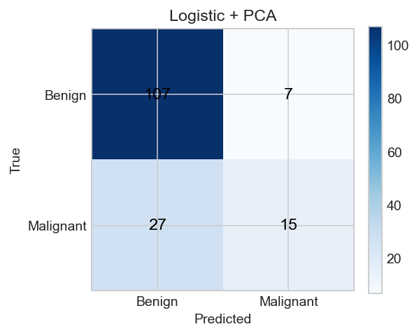
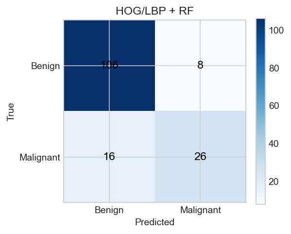
Confusion matrices from the committed training run (same seeds, validation-tuned thresholds):
for fname in ['02_cm_dummy.png', '02_cm_logreg.png', '02_cm_rf.png']:
    display(Image(str(FIG / fname)))
Takeaways#
The dummy’s accuracy is a trap: recall is 0.
PCA-logistic already ranks reasonably (ROC-AUC around 0.80) but is conservative once the F1-tuned threshold is applied — precision over recall.
Hand-crafted edges lift both ranking quality and F1. That is the baseline a CNN has to beat.
Navigation: ← Previous: Images & Labels | Next: Deep Learning →