Fourier Analysis & Spectral Methods#
Navigation: ← Previous: Holt-Winters | Next: ARMA & ARIMA →
Fourier analysis decomposes a series into sinusoids at different frequencies, revealing periodic structure and enabling flexible seasonal regression.
from pathlib import Path
import pandas as pd
import numpy as np
import matplotlib.pyplot as plt
import warnings
warnings.filterwarnings('ignore')
plt.style.use('seaborn-v0_8-whitegrid')

DATA_DIR = Path('data')
if not DATA_DIR.exists():
    DATA_DIR = Path('projects/time-series-analysis/data')

def load_series(name):
    """Load a bundled CSV as a DatetimeIndex Series."""
    df = pd.read_csv(DATA_DIR / name, parse_dates=['date'])
    return df.set_index('date')['value'].sort_index()

def load_air_passengers():
    path = DATA_DIR / 'air_passengers.csv'
    if path.exists():
        return load_series('air_passengers.csv')
    from statsmodels.datasets import get_rdataset
    air = get_rdataset('AirPassengers', 'datasets').data
    s = air['value']
    s.index = pd.date_range('1949-01', periods=len(s), freq='MS')
    return s

def load_milk():
    path = DATA_DIR / 'monthly_milk.csv'
    if path.exists():
        return load_series('monthly_milk.csv')
    url = 'https://raw.githubusercontent.com/jbrownlee/Datasets/master/monthly-milk-production-pounds.csv'
    return pd.read_csv(url, index_col=0, parse_dates=True).squeeze()

def load_co2():
    from statsmodels.datasets import co2
    return co2.load().data.resample('MS').mean().ffill().squeeze()

def load_sunspots():
    from statsmodels.datasets import sunspots
    d = sunspots.load_pandas().data
    return d.set_index('YEAR')['SUNACTIVITY']

def load_retail():
    path = DATA_DIR / 'uk_retail_sales.csv'
    if path.exists():
        return load_series('uk_retail_sales.csv')
    raise FileNotFoundError('uk_retail_sales.csv not found in data/')
import statsmodels.formula.api as smf
from scipy.signal import welch, periodogram
Discrete Fourier Transform#
The DFT maps a series to frequency domain: \(X_k = \sum_{t=0}^{N-1} x_t e^{-2\pi i k t / N}\).
def manual_dft(x):
    N = len(x)
    k = np.arange(N // 2 + 1)
    t = np.arange(N)
    return np.array([np.sum(x * np.exp(-2j * np.pi * k_i * t / N)) for k_i in k])

co2 = load_co2().dropna().values[-120:]  # last 10 years
dft_manual = manual_dft(co2 - co2.mean())
dft_numpy = np.fft.rfft(co2 - co2.mean())
np.allclose(np.abs(dft_manual), np.abs(dft_numpy), rtol=1e-10)
True
# Periodogram of CO2 and Air Passengers
fig, axes = plt.subplots(1, 2, figsize=(12, 5))
for ax, (s, title) in zip(axes, [(load_co2().dropna(), 'Mauna Loa CO2'), (load_air_passengers(), 'Air Passengers')]):
    y = s.values - s.values.mean()
    freqs, psd = periodogram(y, fs=12 if 'CO2' in title or 'Passengers' in title else 1)
    ax.semilogy(freqs, psd)
    ax.set_title(f'Periodogram: {title}')
    ax.set_xlabel('Frequency (cycles per year)')
    ax.set_ylabel('Power')
fig.tight_layout()
fig
Welch’s Method#
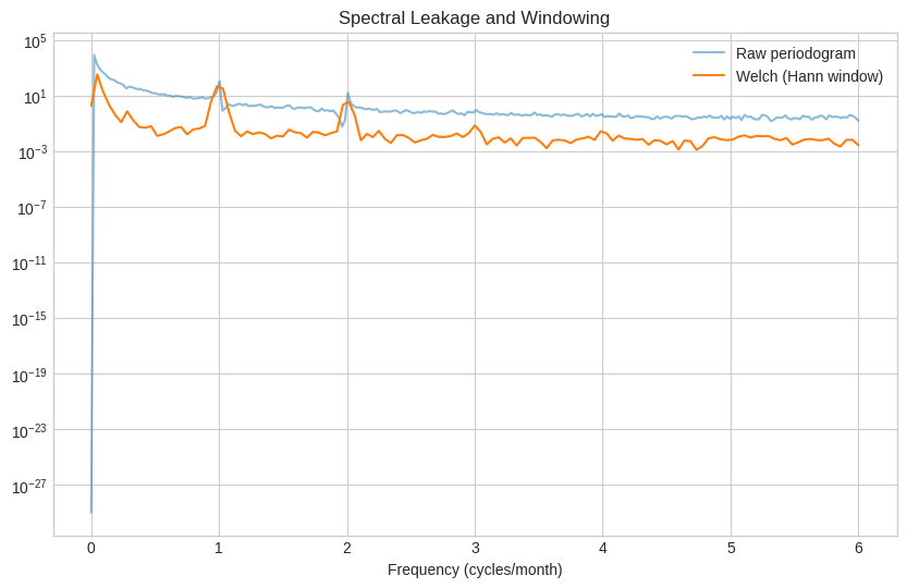
Windowing (Hann) reduces spectral leakage compared to the raw periodogram.
co2_vals = load_co2().dropna().values
f_raw, p_raw = periodogram(co2_vals - co2_vals.mean(), fs=12)
f_welch, p_welch = welch(co2_vals - co2_vals.mean(), fs=12, window='hann', nperseg=256)
fig, ax = plt.subplots(figsize=(10, 6))
ax.semilogy(f_raw, p_raw, alpha=0.5, label='Raw periodogram')
ax.semilogy(f_welch, p_welch, label='Welch (Hann window)')
ax.set_xlabel('Frequency (cycles/month)')
ax.legend()
ax.set_title('Spectral Leakage and Windowing')
fig
Fourier Regressors#
Flexible seasonality via \(K\) pairs of \(\sin, \cos\) terms at harmonics of period \(m\).
def fourier_features(n, period=12, K=3):
    t = np.arange(n)
    cols = {}
    for k in range(1, K + 1):
        cols[f'sin_{k}'] = np.sin(2 * np.pi * k * t / period)
        cols[f'cos_{k}'] = np.cos(2 * np.pi * k * t / period)
    return pd.DataFrame(cols)

co2_s = load_co2().dropna()
n = len(co2_s)
X = fourier_features(n, period=12, K=3)
X['trend'] = np.arange(n)
X['y'] = co2_s.values
model = smf.ols('y ~ trend + sin_1 + cos_1 + sin_2 + cos_2 + sin_3 + cos_3', data=X).fit()
print(model.summary().tables[1])
==============================================================================
                 coef    std err          t      P>|t|      [0.025      0.975]
------------------------------------------------------------------------------
Intercept    310.3767      0.163   1900.943      0.000     310.056     310.697
trend          0.1114      0.001    206.866      0.000       0.110       0.112
sin_1          1.6843      0.116     14.568      0.000       1.457       1.911
cos_1          2.1645      0.116     18.722      0.000       1.937       2.392
sin_2          0.0459      0.116      0.397      0.692      -0.181       0.273
cos_2         -0.7481      0.115     -6.477      0.000      -0.975      -0.521
sin_3          0.0952      0.116      0.823      0.411      -0.132       0.322
cos_3          0.0508      0.116      0.439      0.661      -0.176       0.278
==============================================================================
Key Takeaways#
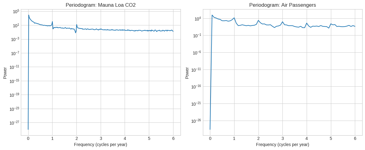
Dominant frequencies: CO₂ shows strong annual cycle (freq ≈ 1/12); Air Passengers shows trend + season.
Windowing: Raw periodograms are noisy; Welch smoothing with Hann window improves estimation.
Fourier regression: Flexible alternative to fixed seasonal dummies; trade-off controlled by \(K\).
Limitation: Assumes fixed seasonal period — inappropriate when seasonality evolves.
Navigation: ← Previous: Holt-Winters | Next: ARMA & ARIMA →