Introduction

Introduction#

A SpatRaster from the terra package stores one or more gridded layers. Each layer is a matrix of cell values aligned to a common extent, resolution, and coordinate reference system (CRS). When a raster has multiple layers—such as twelve monthly temperature grids—each layer is like a variable measured at the same locations on the Earth’s surface.

tidyterra extends dplyr-style verbs to SpatRaster and SpatVector objects. Unlike applying dplyr to a plain data frame, tidyterra::mutate(), select(), and rename() on a raster return another SpatRaster (or updated raster), preserving spatial metadata. That keeps workflows inside the terra object model instead of melting everything to long tables first.

uk_elev <- geodata::elevation_30s(country = "GBR", path = tempdir())
uk_boundary <- rnaturalearth::ne_countries(
  country = "United Kingdom",
  scale = "medium",
  returnclass = "sv"
)

if (!terra::same.crs(uk_elev, uk_boundary)) {
  uk_boundary <- terra::project(uk_boundary, uk_elev)
}

uk_elev_cropped <- terra::crop(uk_elev, uk_boundary)
uk_elev_masked <- terra::mask(uk_elev_cropped, uk_boundary)

elev_layer <- names(uk_elev_masked)[1]
uk_elev_masked <- uk_elev_masked |>
  tidyterra::rename(elevation = !!rlang::sym(elev_layer)) |>
  tidyterra::mutate(
    elev_band = cut(
      elevation,
      breaks = c(-Inf, 100, 300, 600, Inf),
      labels = c("0-100 m", "100-300 m", "300-600 m", "600+ m"),
      include.lowest = TRUE
    )
  )

Cached as: /tmp/Rtmp2iURmb/elevation/GBR_elv_msk.zip

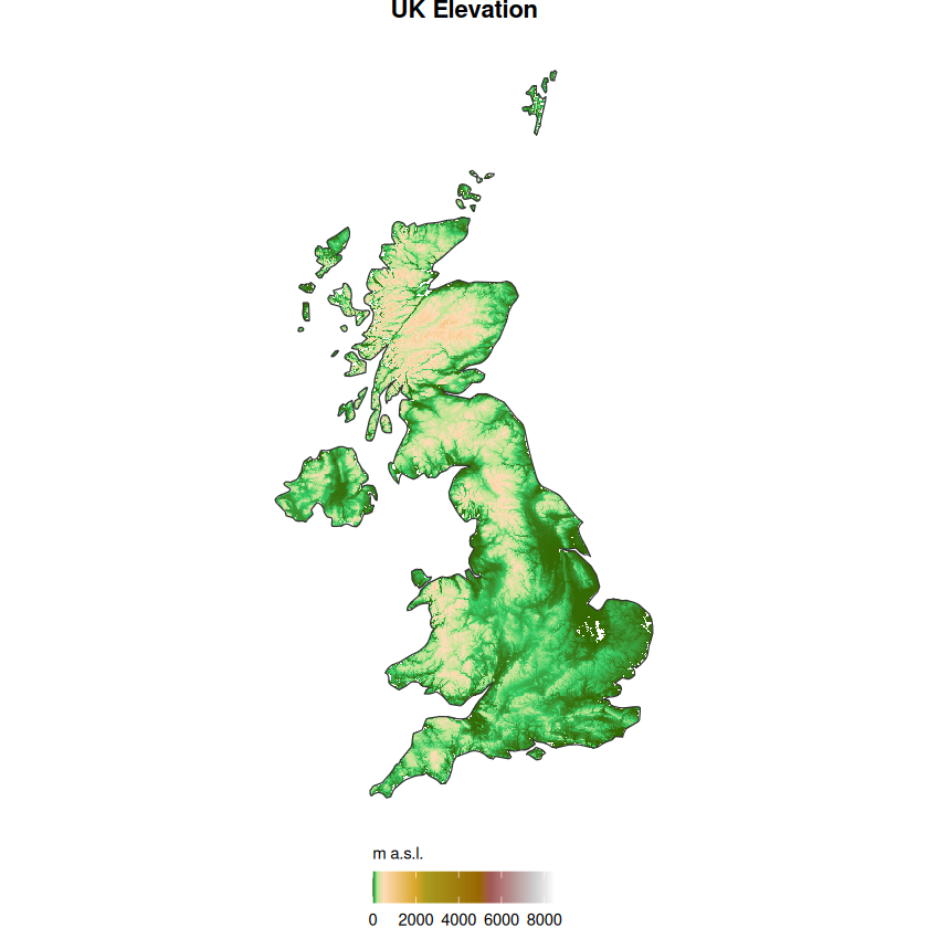
The code above downloads a 30 arc-second (~1 km) elevation grid for Great Britain, clips it to the Natural Earth United Kingdom polygon, and uses terra::crop and terra::mask so only cells inside the national boundary contribute to the map. (Geometric clipping lives in terra; tidyterra is used for dplyr-style layer operations such as rename and mutate.) A numeric layer elevation (metres) is used for continuous mapping; elev_band is a derived categorical layer created with cut() inside mutate(), illustrating dplyr-like syntax on a SpatRaster without dropping the grid structure.

Hypsometric tint palettes mimic cartographic conventions for relief: low elevations read as greens and yellows, high ground as browns and whites. That perceptual ordering matches how people interpret terrain on topographic maps, so scale_fill_hypso_tint_c() is a natural choice for continuous elevation—even when we also keep discrete bands for other summaries.

p_elev <- ggplot() +
  tidyterra::geom_spatraster(data = uk_elev_masked, aes(fill = elevation)) +
  tidyterra::scale_fill_hypso_tint_c(
    name = "m a.s.l.",
    guide = guide_colorbar(barwidth = unit(3.5, "cm"), title.position = "top")
  ) +
  tidyterra::geom_spatvector(data = uk_boundary, fill = NA, colour = "grey20", linewidth = 0.35) +
  labs(title = "UK Elevation") +
  theme_void() +
  theme(
    plot.title = element_text(hjust = 0.5, face = "bold", margin = margin(b = 6)),
    legend.title = element_text(size = 9),
    legend.position = "bottom"
  )

p_elev

<SpatRaster> resampled to 500980 cells.

../../_images/f52dab5f47aa2652fa1b723a0343008d47d3eeea071e1a90a5ee670be30ee9d7.png

Seasonal mean temperature#

WorldClim monthly mean temperature for the UK arrives as a twelve-layer SpatRaster (one layer per month). Layers are indexed 1–12 for January–December. We keep four representative months—December (12), March (3), June (6), September (9)—as proxies for meteorological winter, spring, summer, and autumn in the Northern Hemisphere.

tavg <- geodata::worldclim_country(country = "GBR", var = "tavg", res = 10, path = tempdir())

layer_names <- names(tavg)
season_pick <- layer_names[c(12L, 3L, 6L, 9L)]

uk_tavg_seasons <- tavg |>
  tidyterra::select(dplyr::all_of(season_pick)) |>
  tidyterra::rename(
    Winter = !!rlang::sym(season_pick[1]),
    Spring = !!rlang::sym(season_pick[2]),
    Summer = !!rlang::sym(season_pick[3]),
    Autumn = !!rlang::sym(season_pick[4])
  )

Cached as: /tmp/Rtmp2iURmb/climate/wc2.1_country/GBR_wc2.1_30s_tavg.tif

Here tidyterra::select() subsets raster layers by name (analogous to choosing columns). rename() gives human-readable season labels while the result remains a SpatRaster suitable for geom_spatraster() and faceting.

The whitebox-derived continuous palettes (here "muted") provide colour ramps tuned for terrain and climate-style surfaces; they offer an alternative to hypsometric tints when the variable is temperature rather than relief.

ggplot() +
  tidyterra::geom_spatraster(data = uk_tavg_seasons, aes(fill = after_stat(value))) +
  facet_wrap(~lyr, ncol = 2) +
  tidyterra::scale_fill_whitebox_c(
    palette = "muted",
    name = "°C",
    guide = guide_colorbar(barwidth = unit(2.8, "cm"), title.position = "top")
  ) +
  tidyterra::geom_spatvector(data = uk_boundary, fill = NA, colour = "grey35", linewidth = 0.25) +
  labs(title = "UK Mean Temperature by Season (°C)") +
  theme_void() +
  theme(
    plot.title = element_text(hjust = 0.5, face = "bold", margin = margin(b = 8)),
    strip.text = element_text(face = "bold", size = 10),
    legend.title = element_text(size = 9),
    legend.position = "bottom"
  )

<SpatRaster> resampled to 5e+05 cells.

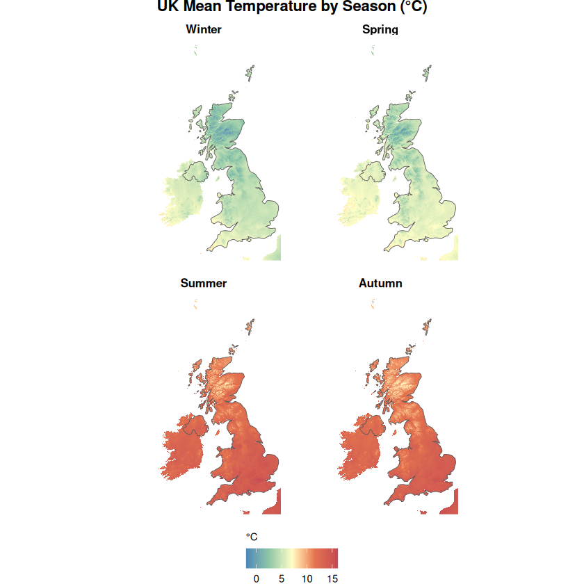
../../_images/f59474cfd4b759901b50763fd9759236f9389563c307f59214ff8f3b7a418ee7.png

Together, the elevation and temperature maps show how multi-layer rasters encode space × variable × time (or season), and how tidyterra keeps those structures intact while integrating with ggplot2.

Introduction

Contents

Introduction#

Seasonal mean temperature#