Evaluation

Navigation: ← Previous: Interpretation | Next: Project Overview →

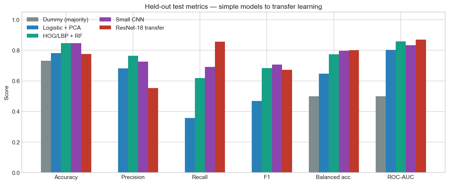
Held-out comparison: accuracy, precision, recall, F1, specificity, ROC/PR, Brier score, and MCC.

What to trust on an imbalanced medical task

Metric	What it answers
Accuracy	Overall hit rate. Inflated by the 73% benign majority.
Precision (PPV)	Of scans flagged malignant, how many are?
Recall (sensitivity)	Of true cancers, how many did we catch?
Specificity	Of benign scans, how many did we leave unflagged?
F1	Harmonic mean of precision and recall; used to pick thresholds on val.
Balanced accuracy	Mean of recall and specificity; chance is 0.5.
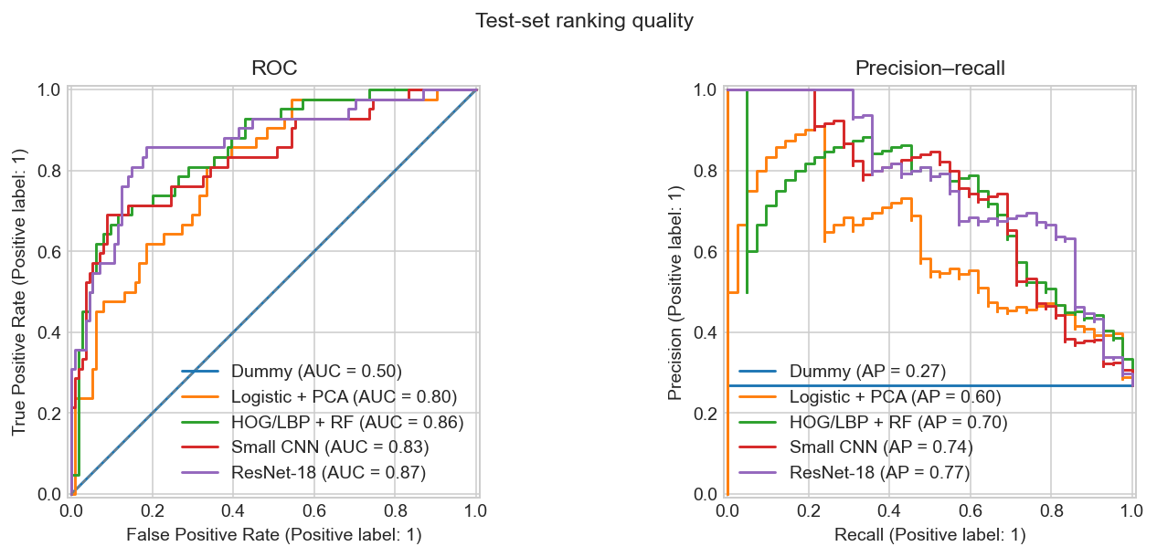
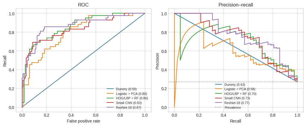
ROC-AUC	Ranking quality across all thresholds.
PR-AUC	Ranking quality with emphasis on the positive class.
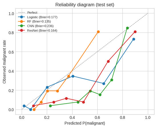
Brier	Mean squared error of predicted probabilities (lower is better).
MCC	Correlation between predictions and labels; 0 is chance.

There is no single winner. A screening-style reader may prefer recall; a second-reader tool may prefer precision. The dummy model makes that tension obvious.

import sys
from pathlib import Path
import numpy as np
import pandas as pd
import matplotlib.pyplot as plt
import warnings
warnings.filterwarnings("ignore")
plt.style.use("seaborn-v0_8-whitegrid")

PROJ_DIR = Path(".").resolve()
if not (PROJ_DIR / "cancer_cv_utils.py").exists():
    PROJ_DIR = Path("projects/cancer-imaging").resolve()
if str(PROJ_DIR) not in sys.path:
    sys.path.insert(0, str(PROJ_DIR))

from cancer_cv_utils import (
    CLASS_NAMES,
    METRIC_ORDER,
    artifacts_dir,
    classification_metrics,
    display_plotly,
    extract_cv_features,
    figures_dir,
    grouped_importance,
    load_metrics,
    load_predictions,
    load_splits,
    metrics_frame,
    overlay_heatmap,
    tune_threshold,
)

SPLITS = load_splits()
FIG = figures_dir()
ART = artifacts_dir()
print("Splits:", {k: v["labels"].shape[0] for k, v in SPLITS.items()})
print("Malignant rates:", {k: f"{v['labels'].mean():.1%}" for k, v in SPLITS.items()})

Splits: {'train': 546, 'val': 78, 'test': 156}
Malignant rates: {'train': '26.9%', 'val': '26.9%', 'test': '26.9%'}

mets = load_metrics()
preds = load_predictions()
table = metrics_frame(mets).round(3)
table

	accuracy	precision	recall	f1	specificity	balanced_accuracy	roc_auc	pr_auc	brier	mcc
model
Dummy (majority)	0.731	0.000	0.000	0.000	1.000	0.500	0.500	0.269	0.269	0.000
Logistic + PCA	0.782	0.682	0.357	0.469	0.939	0.648	0.802	0.599	0.177	0.377
HOG/LBP + RF	0.846	0.765	0.619	0.684	0.930	0.774	0.858	0.703	0.135	0.590
Small CNN	0.846	0.725	0.690	0.707	0.904	0.797	0.833	0.736	0.236	0.603
ResNet-18 transfer	0.776	0.554	0.857	0.673	0.746	0.801	0.869	0.772	0.164	0.542

Interactive metric table

import plotly.graph_objects as go
show = table.reset_index().rename(columns={'model': 'Model'})
fig = go.Figure(data=[go.Table(
    header=dict(values=list(show.columns), fill_color='#0b3d4a', font=dict(color='white')),
    cells=dict(values=[show[c] for c in show.columns], align='left'),
)])
fig.update_layout(margin=dict(l=0, r=0, t=8, b=8), height=280)
display_plotly(fig)

Bars and ranking curves

from IPython.display import Image, display
display(Image(str(FIG / '05_metrics_bars.png')))
display(Image(str(FIG / '05_roc_pr.png')))

ROC and precision–recall from stored test probabilities

from sklearn.metrics import precision_recall_curve, roc_curve, auc as sk_auc

y = preds['y_true']
series = [
    ('Dummy', preds['dummy']),
    ('Logistic + PCA', preds['logreg']),
    ('HOG/LBP + RF', preds['rf']),
    ('Small CNN', preds['cnn']),
    ('ResNet-18', preds['resnet']),
]
fig, axes = plt.subplots(1, 2, figsize=(10.5, 4.4))
for name, prob in series:
    fpr, tpr, _ = roc_curve(y, prob)
    prec, rec, _ = precision_recall_curve(y, prob)
    axes[0].plot(fpr, tpr, label=f'{name} ({sk_auc(fpr, tpr):.2f})')
    axes[1].plot(rec, prec, label=f'{name} ({sk_auc(rec, prec):.2f})')
axes[0].plot([0, 1], [0, 1], ls='--', c='grey', lw=0.8)
axes[0].set_xlabel('False positive rate'); axes[0].set_ylabel('Recall')
axes[0].set_title('ROC')
axes[1].set_xlabel('Recall'); axes[1].set_ylabel('Precision')
axes[1].set_title('Precision–recall')
axes[1].axhline(y.mean(), ls=':', c='grey', label='Prevalence')
for ax in axes:
    ax.legend(frameon=False, fontsize=8)
fig.tight_layout()
plt.show()

Calibration (Brier and reliability)

from sklearn.calibration import calibration_curve

brier_of = {
    'Logistic': mets['Logistic + PCA']['brier'],
    'RF': mets['HOG/LBP + RF']['brier'],
    'CNN': mets['Small CNN']['brier'],
    'ResNet': mets['ResNet-18 transfer']['brier'],
}
fig, ax = plt.subplots(figsize=(5.6, 4.6))
ax.plot([0, 1], [0, 1], ls='--', c='grey', lw=0.8, label='Perfect')
for name, key in [('Logistic', 'logreg'), ('RF', 'rf'), ('CNN', 'cnn'), ('ResNet', 'resnet')]:
    frac, meanp = calibration_curve(y, preds[key], n_bins=6, strategy='quantile')
    ax.plot(meanp, frac, marker='o', label=f'{name} (Brier={brier_of[name]:.3f})')
ax.set_xlabel('Predicted P(malignant)')
ax.set_ylabel('Observed malignant rate')
ax.set_title('Reliability diagram (test set)')
ax.legend(frameon=False, fontsize=8)
plt.tight_layout()
plt.show()

Error counts at the chosen thresholds

False negatives are missed cancers; false positives are extra work for a human reader.

err = pd.DataFrame({
    name: {'TP': m['tp'], 'FP': m['fp'], 'TN': m['tn'], 'FN': m['fn'], 'threshold': m['threshold']}
    for name, m in mets.items()
}).T
err

	TP	FP	TN	FN	threshold
Dummy (majority)	0.0	0.0	114.0	42.0	0.5
Logistic + PCA	15.0	7.0	107.0	27.0	0.8
HOG/LBP + RF	26.0	8.0	106.0	16.0	0.4
Small CNN	29.0	11.0	103.0	13.0	0.7
ResNet-18 transfer	36.0	29.0	85.0	6.0	0.5

What improved?

• Dummy → logistic: ranking appears (ROC-AUC ~0.80). Accuracy barely moves; recall is no longer zero.

• Logistic → HOG/LBP forest: best precision of the ladder, strong accuracy and AUC. Classical CV still earns its keep on a small dataset.

• Forest → small CNN: similar accuracy, slightly higher F1 and PR-AUC, worse Brier (probabilities are less calibrated).

• CNN → ResNet-18 transfer: highest ROC-AUC and PR-AUC and the fewest missed cancers (FN), at the cost of more false positives and lower accuracy than the forest.

On 156 test images these gaps are noisy. The honest summary is: engineered edges beat raw pixels; transfer learning is the best ranker and the most sensitive detector; no model is ready for clinic. Domain shift, 128px resolution, and a single-source ultrasound set are hard limits.

Rebuild

python projects/cancer-imaging/_prepare_data.py   # if the NPZ is missing
python projects/cancer-imaging/_train_models.py   # regenerate weights and figures
python projects/cancer-imaging/_generate_notebooks.py

---

Navigation: ← Previous: Interpretation | Next: Project Overview →