Introduction to State-Space & Structural Models#
Navigation: ← Previous: SARIMA | Next: Model Comparison →
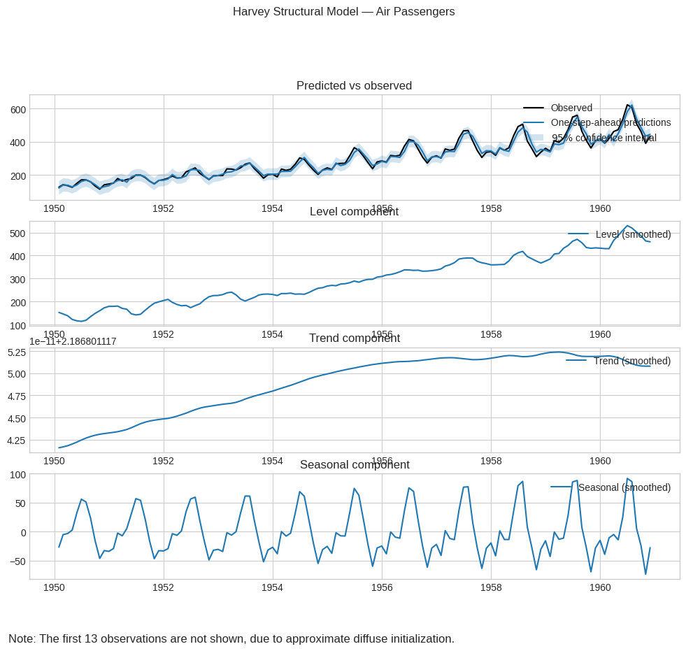
State-space models separate observed data from unobserved components (level, trend, season), estimated via the Kalman filter.
from pathlib import Path
import pandas as pd
import numpy as np
import matplotlib.pyplot as plt
import warnings
warnings.filterwarnings('ignore')
plt.style.use('seaborn-v0_8-whitegrid')

DATA_DIR = Path('data')
if not DATA_DIR.exists():
    DATA_DIR = Path('projects/time-series-analysis/data')

def load_series(name):
    """Load a bundled CSV as a DatetimeIndex Series."""
    df = pd.read_csv(DATA_DIR / name, parse_dates=['date'])
    return df.set_index('date')['value'].sort_index()

def load_air_passengers():
    path = DATA_DIR / 'air_passengers.csv'
    if path.exists():
        return load_series('air_passengers.csv')
    from statsmodels.datasets import get_rdataset
    air = get_rdataset('AirPassengers', 'datasets').data
    s = air['value']
    s.index = pd.date_range('1949-01', periods=len(s), freq='MS')
    return s

def load_milk():
    path = DATA_DIR / 'monthly_milk.csv'
    if path.exists():
        return load_series('monthly_milk.csv')
    url = 'https://raw.githubusercontent.com/jbrownlee/Datasets/master/monthly-milk-production-pounds.csv'
    return pd.read_csv(url, index_col=0, parse_dates=True).squeeze()

def load_co2():
    from statsmodels.datasets import co2
    return co2.load().data.resample('MS').mean().ffill().squeeze()

def load_sunspots():
    from statsmodels.datasets import sunspots
    d = sunspots.load_pandas().data
    return d.set_index('YEAR')['SUNACTIVITY']

def load_retail():
    path = DATA_DIR / 'uk_retail_sales.csv'
    if path.exists():
        return load_series('uk_retail_sales.csv')
    raise FileNotFoundError('uk_retail_sales.csv not found in data/')
from statsmodels.tsa.statespace.structural import UnobservedComponents
State-Space Form#
Observation: \(y_t = Z_t \alpha_t + \varepsilon_t\). State: \(\alpha_{t+1} = T_t \alpha_t + R_t \eta_t\).
Local level \(\equiv\) ARIMA(0,1,1). Local linear trend \(\equiv\) ARIMA(0,2,2).
air = load_air_passengers()

# Local level model
uc_level = UnobservedComponents(air, level='local level').fit(disp=False)
print('Local level AIC:', uc_level.aic)

# Local linear trend + seasonal
uc_struct = UnobservedComponents(
    air, level='local linear trend', seasonal=12
).fit(disp=False)
print('Structural (trend+season) AIC:', uc_struct.aic)
/opt/hostedtoolcache/Python/3.11.16/x64/lib/python3.11/site-packages/statsmodels/tsa/base/tsa_model.py:480: ValueWarning: No frequency information was provided, so inferred frequency MS will be used.
  self._init_dates(dates, freq)
/opt/hostedtoolcache/Python/3.11.16/x64/lib/python3.11/site-packages/statsmodels/tsa/base/tsa_model.py:480: ValueWarning: No frequency information was provided, so inferred frequency MS will be used.
  self._init_dates(dates, freq)
Local level AIC: 1415.9091174925184
Structural (trend+season) AIC: 1140.1026158818113
# Extract components
fig = uc_struct.plot_components(figsize=(12, 9))
fig.suptitle('Harvey Structural Model — Air Passengers', y=1.02)
fig
ARIMA Equivalences#
Structural model |
Equivalent ARIMA |
|---|---|
Local level |
ARIMA(0,1,1) |
Local linear trend |
ARIMA(0,2,2) |
Local level + seasonal(12) |
ARIMA(0,1,1)(0,1,1)₁₂ |
Production tools: KFAS (R), statsmodels (Python), used internally by TRAMO-SEATS and JDemetra+.
Key Takeaways#
Interpretability: Structural models decompose into level, trend, season — unlike black-box ARIMA.
Kalman filter: Optimal recursive estimation under Gaussian linear assumptions.
Equivalence: Many ARIMA models have structural representations — choose based on purpose.
Missing data: State-space handles gaps naturally; ARIMA requires complete series.
Navigation: ← Previous: SARIMA | Next: Model Comparison →