Fay–Herriot: classical EBLUP#
Navigation: ← Previous: Direct Estimates | Next: Bayesian Hierarchical Model →
REML fit of \(\sigma_u^2\), EBLUP shrinkage, Prasad–Rao / Datta–Lahiri MSE, and a delete-one jackknife — the same objects as sae::eblupFH / emdi::fh.
import sys
from pathlib import Path
import pandas as pd
import numpy as np
import matplotlib.pyplot as plt
import plotly.graph_objects as go
import plotly.express as px
from IPython.display import HTML, display
import warnings
warnings.filterwarnings('ignore')
plt.style.use('seaborn-v0_8-whitegrid')

PROJ_DIR = Path('.').resolve()
if not (PROJ_DIR / 'sae_utils.py').exists():
    PROJ_DIR = Path('projects/small-area-estimation').resolve()
if str(PROJ_DIR) not in sys.path:
    sys.path.insert(0, str(PROJ_DIR))

from sae_utils import (
    load_panel, modelling_frame, design_matrix, eblup_fh, fh_reml_sigma_u,
    jackknife_mse, gibbs_fh, summarise_theta, posterior_predictive_y,
    rhat_split, coverage_rate, project_data_dir,
)

def display_plotly(fig):
    """Embed Plotly with CDN JS — fig.show() is blank in Jupyter Book HTML."""
    display(HTML(fig.to_html(include_plotlyjs='cdn', full_html=False)))

FIG_DIR = PROJ_DIR / 'figures'
FIG_DIR.mkdir(exist_ok=True)
DATA_DIR = project_data_dir()
PANEL = load_panel()
MODEL = modelling_frame(PANEL)
print(f'Panel: {len(PANEL)} local authorities; modelling subset: {len(MODEL)}')
print(f'Period (APS / ONS model-based): {PANEL["direct_period"].dropna().iloc[0]}')
Panel: 348 local authorities; modelling subset: 136
Period (APS / ONS model-based): Apr 2025-Mar 2026
The frequentist target#
Stacking the sampling and linking models gives the marginal
REML maximises the residual likelihood after projecting out \(\beta\) (Rao & Molina, 2015, §5.2). Given \(\hat{\sigma}_u^2\), GLS supplies \(\hat{\beta}\) and the EBLUP \(\hat{\theta}_i = \hat{\gamma}_i y_i + (1-\hat{\gamma}_i) x_i'\hat{\beta}\).
We implement this in sae_utils.eblup_fh rather than wrapping R. The algebra is that of sae::eblupFH(..., method = "REML") and emdi::fh(..., method = "reml"): known \(\psi_i\), linear mean, independent random effects. What we do not include is emdi’s spatial/temporal extensions or automatic transformation of \(y\).
fit = eblup_fh(MODEL, covariates=['claimant_rate'])
info = fit.attrs['fit']
print('REML σ²_u = {:.3f}  (σ_u = {:.3f})'.format(info['sigma_u2'], info['sigma_u']))
print('MOM start  = {:.3f}'.format(info['mom_start']))
print('converged  =', info['converged'])
print('Var(σ²_u)  = {:.3f}'.format(info['var_sigma_u2']))
beta = np.array(info['beta'])
for name, b in zip(info['coef_names'], beta):
    print(f'  β[{name}] = {b:.3f}')
print(f"\nmedian γ = {fit['gamma'].median():.3f}  "
      f"min={fit['gamma'].min():.3f}  max={fit['gamma'].max():.3f}")
fit[['GEOGRAPHY_NAME','direct_rate','eblup','gamma','eblup_se','ons_mb_rate']].head(8)
REML σ²_u = 0.956  (σ_u = 0.978)
MOM start  = 1.020
converged  = True
Var(σ²_u)  = 0.075
  β[intercept] = 2.408
  β[claimant_rate] = 0.646

median γ = 0.410  min=0.154  max=0.752
| GEOGRAPHY_NAME | direct_rate | eblup | gamma | eblup_se | ons_mb_rate | |
|---|---|---|---|---|---|---|
| 0 | Barking and Dagenham | 6.1 | 6.921328 | 0.289883 | 0.872491 | 8.2 |
| 1 | Barnet | 5.5 | 5.593416 | 0.335095 | 0.818572 | 5.9 |
| 2 | Barnsley | 2.6 | 3.337420 | 0.620187 | 0.616751 | 3.8 |
| 3 | Bath and North East Somerset | 4.6 | 4.097790 | 0.478758 | 0.730763 | 3.9 |
| 4 | Bexley | 7.3 | 5.176156 | 0.211586 | 0.887394 | 5.5 |
| 5 | Birmingham | 8.5 | 8.668065 | 0.454476 | 0.796043 | 8.1 |
| 6 | Blackburn with Darwen | 4.3 | 5.099809 | 0.478758 | 0.726022 | 5.3 |
| 7 | Blackpool | 4.2 | 5.355193 | 0.478758 | 0.730830 | 4.7 |
MSE: \(g_1 + g_2 + 2g_3\)#
Prasad & Rao (1990) decompose the EBLUP MSE. Datta & Lahiri (2000) show that for REML the leading correction is twice \(g_3\):
\(g_1 = \gamma_i \psi_i\) — leading term, the posterior variance if \(\beta,\sigma_u^2\) were known;
\(g_2\) — uncertainty in \(\hat\beta\);
\(g_3\) — uncertainty in \(\hat\sigma_u^2\), involving \(\widehat{\mathrm{Var}}(\hat\sigma_u^2) = 2 / \mathrm{tr}(P_V^2)\).
These are model-based MSEs. They understate error if the linking model is misspecified, and they ignore uncertainty in \(\psi_i\).
print(fit[['eblup_mse','eblup_se']].describe().round(3).to_string())
print('\nMedian SE: direct CI/1.96 vs EBLUP')
print(pd.DataFrame({
    'direct_se': MODEL['direct_rate_ci']/1.96,
    'eblup_se': fit['eblup_se'],
}).median().round(3))
       eblup_mse  eblup_se
count    136.000   136.000
mean       0.601     0.770
std        0.138     0.093
min        0.247     0.497
25%        0.524     0.724
50%        0.598     0.773
75%        0.700     0.837
max        0.895     0.946

Median SE: direct CI/1.96 vs EBLUP
direct_se    1.173
eblup_se     0.773
dtype: float64
Jackknife MSE#
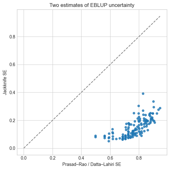
Jiang, Lahiri & Wan (2002) jackknife the EBLUP by deleting one area at a time and refitting \(\sigma_u^2\). We report the jackknife variance of the EBLUP as a check on \(g_1+g_2+2g_3\), not as a replacement: with \(m \approx 100\) areas the delete-one perturbation of \(\hat\sigma_u^2\) is noisy, and the two estimators can diverge in the tails.
jack_var = jackknife_mse(MODEL, covariates=['claimant_rate'])
fit = fit.copy()
fit['eblup_se_jack'] = np.sqrt(np.maximum(jack_var, 0))
print(fit[['eblup_se','eblup_se_jack']].describe().round(3).to_string())
fig, ax = plt.subplots(figsize=(5.5, 5.5))
ax.scatter(fit['eblup_se'], fit['eblup_se_jack'], s=22, alpha=0.8)
mmax = max(fit['eblup_se'].max(), fit['eblup_se_jack'].max())
ax.plot([0, mmax], [0, mmax], '--', color='grey')
ax.set_xlabel('Prasad–Rao / Datta–Lahiri SE')
ax.set_ylabel('Jackknife SE')
ax.set_title('Two estimates of EBLUP uncertainty')
fig.tight_layout()
fig.savefig(FIG_DIR / '04_mse_jackknife.png', dpi=120)
fig
       eblup_se  eblup_se_jack
count   136.000        136.000
mean      0.770          0.150
std       0.093          0.067
min       0.497          0.051
25%       0.724          0.092
50%       0.773          0.135
75%       0.837          0.196
max       0.946          0.393
Shrinkage in the data#
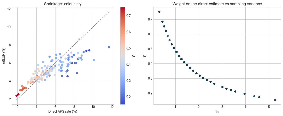
Plot \(y_i\) against the EBLUP. Points far from \(y=x\) are the areas the model is willing to move; they should be the high-\(\psi_i\) ones.
fig, axes = plt.subplots(1, 2, figsize=(12, 5))
sc = axes[0].scatter(fit['direct_rate'], fit['eblup'], c=fit['gamma'], cmap='coolwarm', s=32)
lims = [fit[['direct_rate','eblup']].min().min(), fit[['direct_rate','eblup']].max().max()]
axes[0].plot(lims, lims, '--', color='grey')
axes[0].set_xlabel('Direct APS rate (%)')
axes[0].set_ylabel('EBLUP (%)')
axes[0].set_title('Shrinkage: colour = γ')
fig.colorbar(sc, ax=axes[0], label=r'$\gamma_i$')
axes[1].scatter(fit['psi'], fit['gamma'], s=28, alpha=0.8, c='#0d3b4c')
axes[1].set_xlabel(r'$\psi_i$')
axes[1].set_ylabel(r'$\gamma_i$')
axes[1].set_title('Weight on the direct estimate vs sampling variance')
fig.tight_layout()
fig.savefig(FIG_DIR / '04_shrinkage.png', dpi=120)
fig
Adding inactivity#
A second covariate (APS inactivity) is itself a survey estimate, so it violates the ‘known \(x\)’ assumption. We fit it as a sensitivity check, not as the preferred specification. If \(\hat\sigma_u^2\) barely moves, claimant count already absorbs most of the between-area signal.
m2 = MODEL.dropna(subset=['inactivity_rate']).copy()
fit2 = eblup_fh(m2, covariates=['claimant_rate', 'inactivity_rate'])
i2 = fit2.attrs['fit']
print('claimant-only σ²_u = {:.3f}'.format(info['sigma_u2']))
print('claimant+inactivity σ²_u = {:.3f}'.format(i2['sigma_u2']))
print('coefficients:', dict(zip(i2['coef_names'], np.round(i2['beta'], 3))))
claimant-only σ²_u = 0.956
claimant+inactivity σ²_u = 0.970
coefficients: {'intercept': np.float64(2.252), 'claimant_rate': np.float64(0.635), 'inactivity_rate': np.float64(0.009)}
Key takeaways#
REML \(\hat\sigma_u^2\) determines the global amount of borrowing; \(\psi_i\) then allocates it locally via \(\gamma_i\).
Datta–Lahiri MSE is the analytic default; the jackknife is a useful disagreement diagnostic, not an automatic upgrade.
Treating a survey covariate as \(x_i\) is a specification error — keep the production-style model to claimant count.
Navigation: ← Previous: Direct Estimates | Next: Bayesian Hierarchical Model →