Power Laws and Popularity

Navigation: ← Project overview · Next: Genre from audio →

What 50,000 synthetic tracks and 500 invented artists can — and cannot — tell you about streaming success.

This page is the analysis. Fitting lives in src/spotify_powerlaws/ and scripts/00_–09_; the Jupyter Book build loads committed artifacts/ so it does not retrain. Rebuild with make all from the project directory.

import json
from pathlib import Path
import pandas as pd
from IPython.display import display

PROJ = Path(".").resolve()
if not (PROJ / "artifacts" / "metrics.json").exists():
    PROJ = Path("projects/spotify-power-laws").resolve()

def load(name):
    return json.loads((PROJ / "artifacts" / name).read_text())

schema = load("schema.json")
forensics = load("forensics.json")
estimand = load("estimand.json")
models = load("models.json")
curve = load("learning_curve.json")
dist = load("distributional.json")
unc = load("uncertainty.json")
metrics = load("metrics.json")

print(f"Rows {schema['n_rows']:,} · columns {schema['n_cols']} · artists {schema['n_artists']}")
print(f"Grain: {schema['grain']}")
print(f"Seed: {metrics['seed']}")

Rows 50,000 · columns 33 · artists 500
Grain: track
Seed: 20260903

1. The file is not what the brief implied

The Kaggle title sounds like an artist panel for 2020–2025. The file is a track catalog: 50,000 rows, unique track_id, 33 columns, 500 invented artist names. release_date covers every calendar day from 2020-01-01 to 2025-12-31. That is a release calendar, not a listening panel, so there is no artist-level streaming series to seasonally adjust.

The publisher already says the data are fully synthetic and that no Spotify API data were used. The rest of this section is the check a reviewer should still run.

ben = forensics["benford_stream_count"]
term = forensics["terminal_stream_count"]
icc_a = forensics["icc_log_streams_artist"]
print("Benford χ² = {:.2f} (df 8, p = {:.2f}); MAD = {:.4f} ({})".format(
    ben["chi2"], ben["p_value"], ben["mad"], ben["nigrini_conformity"]))
print("Terminal-digit χ² p = {:.2f}; share ending 0 = {:.3f} (uniform 0.10)".format(
    term["p_value"], term["share_mod10_zero"]))
print("Known real artists present:", forensics["n_known_real_artists_present"], "of 10")
print("energy–loudness r = {:.3f}".format(forensics["energy_loudness_corr"]))
print("max |audio, streams| r = {:.4f}".format(max(abs(v) for v in forensics["audio_target_correlations"].values())))
print("popularity vs log1p(streams) r = {:.3f}".format(forensics["popularity_log1p_streams_corr"]))
print("Artist ICC on log1p streams = {:.5f}; design effect = {:.3f}; n_eff = {:.0f}".format(
    icc_a["icc"], icc_a["design_effect"], icc_a["n_effective"]))
print("Missing audio:", schema["missing_audio"])
print(forensics["verdict"])

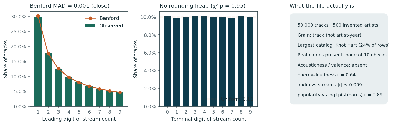
Benford χ² = 4.70 (df 8, p = 0.79); MAD = 0.0009 (close)
Terminal-digit χ² p = 0.95; share ending 0 = 0.101 (uniform 0.10)
Known real artists present: 0 of 10
energy–loudness r = 0.642
max |audio, streams| r = 0.0091
popularity vs log1p(streams) r = 0.894
Artist ICC on log1p streams = -0.00010; design effect = 0.990; n_eff = 50498
Missing audio: ['acousticness', 'valence', 'speechiness', 'liveness', 'time_signature']
The file is a synthetic track catalog with 500 invented artists. Audio features are orthogonal to streams; popularity is a compressed copy of log streams; the superstar pattern is catalog size, not per-track quality. It can teach leakage, validation, and model-capacity questions about this generator. It cannot support claims about Spotify.

What survives. Digit leading-order looks Benford-like (Nigrini MAD 0.001, close conformity). That is what a heavy-tailed generator does; it is not evidence the counts are real. Terminal digits are uniform — no 10/100/1,000 heaping. None of ten household-name artists appear. Acousticness and valence are absent, so the usual Spotify audio-feature checks cannot be finished. Popularity is integer-valued, 0–92 not 0–100, and almost a compressed copy of log1p(stream_count).

What does not survive. Any claim about Spotify, COVID listening, or a named artist’s career. The interesting work is about this generator: leakage, validation, and whether extra model capacity invents a coupling that was never planted.

2. Estimand, then a leakage audit

Target. stream_count, modelled on the log1p scale, back-transformed with Duan’s smearing estimator (\exp(\hat\mu), \overline{\exp(e)} - 1). Popularity is not a second outcome; it is nearly the same variable.

Question. Among tracks in this catalog, what is the association between antecedent audio and release features and log stream counts, with artist as the unit of independence? The predictive rider is whether those features forecast streams for a held-out artist.

Decision. Do not ship a “Spotify success model” trained here. Do not report (R^2) from popularity or log_stream_count as a result about music.

Not identified. Genre, label, or country effects in the real industry; 2020 as an intervention; generalisation to Spotify.

roles = pd.Series(estimand["feature_roles"], name="role").rename_axis("column").reset_index()
print("Honest numeric:", ", ".join(estimand["honest_numeric"]))
print("Honest categorical:", ", ".join(estimand["honest_categorical"]))
print("Leakage arm:", ", ".join(estimand["leakage_numeric"] + estimand["leakage_categorical"]))
display(roles)

Honest numeric: duration_ms, danceability, energy, loudness, instrumentalness, tempo, key, mode, explicit, release_month
Honest categorical: genre, country, label
Leakage arm: popularity, log_stream_count, artist_track_count, popularity_category

	column	role
0	duration_ms	antecedent
1	danceability	antecedent
2	energy	antecedent
3	loudness	antecedent
4	instrumentalness	antecedent
5	tempo	antecedent
6	key	antecedent
7	mode	antecedent
8	explicit	antecedent
9	release_month	antecedent (release calendar)
10	genre	antecedent / concurrent label
11	country	concurrent; origin vs market unidentified
12	label	concurrent; mix of real and invented names
13	upbeat_score	constructed from audio; excluded as duplicate
14	duration_minutes	constructed; excluded as duplicate
15	key_name	constructed; excluded as duplicate
16	mode_name	constructed; excluded as duplicate
17	is_explicit_bool	constructed; excluded as duplicate
18	release_year	constructed from date; excluded (collinear wit...
19	release_quarter	constructed; excluded as duplicate
20	is_weekend_release	constructed; excluded as duplicate of calendar
21	loudness_category	constructed; excluded as duplicate
22	popularity	consequent of streams
23	popularity_category	discretisation of popularity
24	log_stream_count	deterministic transform of the target
25	artist_track_count	whole-sample group size

log_stream_count is round(log1p(stream_count), 4). Putting it in (X) is predicting (y) from (y). artist_track_count is the full-sample group size. upbeat_score is a linear composite of danceability, energy and tempo. Those columns are the leakage arm, not the estimand.

3. Validation has to match the dependence — and the tautology

Two splits, same OLS, two feature sets. Grouped five-fold by artist_name versus shuffled five-fold. Nested comparison uses the Nadeau–Bengio corrected resampled (t)-test on the five outer folds.

rows = []
for label, key in [
    ("Intercept, grouped", "intercept_grouped"),
    ("OLS honest, grouped", "ols_honest_grouped"),
    ("OLS honest, random", "ols_honest_random"),
    ("OLS leakage, grouped", "ols_leakage_grouped"),
    ("OLS leakage, random", "ols_leakage_random"),
    ("Elastic net honest, grouped", "elastic_net"),
    ("HGB honest, grouped", "boosting"),
]:
    block = models[key]["summary"] if key != "elastic_net" else models[key]["summary"]
    rows.append({
        "model": label,
        "RMSE log": block["rmse_log"]["mean"],
        "R² log": block["r2_log"]["mean"],
        "MAE count (Duan)": block["mae_count"]["mean"],
    })
tab = pd.DataFrame(rows).set_index("model")
display(tab.round(4))
print("Grouped vs random honest RMSE relative drop: {:.3%}".format(models["optimism_gap_honest_rmse"]["relative_drop"]))
print("Leakage vs honest grouped R²: {:.3f} vs {:.3f}".format(
    models["leakage_gap_grouped_r2"]["leakage"], models["leakage_gap_grouped_r2"]["honest"]))
for name, test in models["tests"].items():
    print(f"{name}: ΔRMSE = {test['mean_diff']:.4f}, t = {test['t']:.2f}, p = {test['p_value']:.3g}")

	RMSE log	R² log	MAE count (Duan)
model
Intercept, grouped	1.7949	-0.0001	162138.3984
OLS honest, grouped	1.7527	0.0464	148378.2129
OLS honest, random	1.7511	0.0470	147428.5085
OLS leakage, grouped	0.0000	1.0000	2.9539
OLS leakage, random	0.0000	1.0000	2.9286
Elastic net honest, grouped	1.7518	0.0474	148458.9457
HGB honest, grouped	1.7563	0.0425	148363.5915

Grouped vs random honest RMSE relative drop: 0.091%
Leakage vs honest grouped R²: 1.000 vs 0.046
ols_vs_intercept_grouped: ΔRMSE = -0.0422, t = -41.21, p = 2.07e-06
boost_vs_ols_grouped: ΔRMSE = 0.0035, t = 4.15, p = 0.0143
enet_vs_ols_grouped: ΔRMSE = -0.0010, t = -2.11, p = 0.103
ols_random_vs_grouped: ΔRMSE = -0.0016, t = -0.10, p = 0.929
leakage_vs_honest_grouped: ΔRMSE = -1.7527, t = -137.16, p = 1.69e-08

Two results, both expected once the DGP is visible.

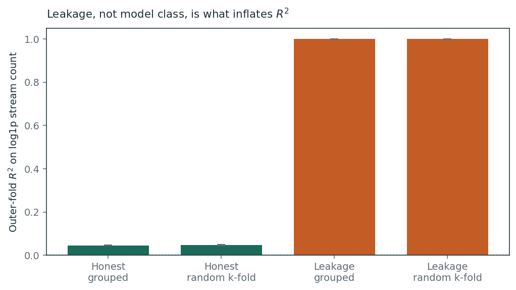
1. Leakage is the whole (R^2). Honest grouped OLS has (R^2 \approx 0.046). The leakage arm has (R^2 = 1) under both split policies, because log_stream_count is the target. Grouped CV does not rescue a tautological feature.

2. Random k-fold does not inflate the honest model. Artist ICC on log1p streams is (\approx 0), so the design effect for a track-level mean is 1. The small-(n) constraint lives at the artist estimand (500 names, one of them 24% of rows), not at the track mean. Showing a null optimism gap is the correct report, not a disappointment.

The learning curve samples training artists, not rows, and scores a fixed panel of 80 held-out artists.

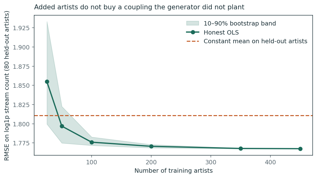
Honest OLS beats a constant after about 50 artists and then saturates. More artists do not buy a coupling the generator did not plant. That is the central constraint, restated for a 50,000-row file that is still a 500-artist problem.

4. Capacity stops paying immediately

Fit in order: intercept, OLS, ridge / elastic net, cubic splines on energy–loudness–danceability, histogram gradient boosting with early stopping, then a random-intercept mixed model by artist.

spl = models["spline_vs_linear"]["paired_test"]
print("Splines vs linear ΔRMSE = {:.5f}, t = {:.2f}, p = {:.2f}".format(spl["mean_diff"], spl["t"], spl["p_value"]))
print("Boosting vs OLS:", models["tests"]["boost_vs_ols_grouped"])
print("Elastic net vs OLS:", models["tests"]["enet_vs_ols_grouped"])
print("MixedLM artist SD = {:.3f}; residual SD = {:.3f}; ICC = {:.4f}; converged = {}".format(
    models["mixedlm"]["sd_artist"],
    models["mixedlm"]["var_resid"] ** 0.5,
    models["mixedlm"]["icc"],
    models["mixedlm"]["converged"],
))

Splines vs linear ΔRMSE = 0.00036, t = 1.12, p = 0.33
Boosting vs OLS: {'mean_diff': 0.003539296989397611, 't': 4.149126712822952, 'df': 4, 'p_value': 0.014270389585734632, 'correction': 'Nadeau-Bengio 2003; n_test/n_train = 1/(k-1)'}
Elastic net vs OLS: {'mean_diff': -0.0009536873870593876, 't': -2.106794711783205, 'df': 4, 'p_value': 0.10286160286219793, 'correction': 'Nadeau-Bengio 2003; n_test/n_train = 1/(k-1)'}
MixedLM artist SD = 0.072; residual SD = 1.793; ICC = 0.0016; converged = False

Elastic net is indistinguishable from OLS. Splines are not better than linear. Boosting is slightly worse (corrected (t = 4.15), (p = 0.014)) — extra capacity fits noise in a DGP where audio is orthogonal to streams. The mixed model puts almost all variance in the residual; optimisation reports a boundary/singular random-effect covariance, which is the ANOVA ICC again. Partial pooling collapses toward complete pooling because there is nothing to pool.

Metrics on the count scale use Duan smearing, not expm1 of the log prediction. Honest MAE is still ~150,000 streams against a median of 16,000: the model is not useful for counts, and pretending otherwise would be the usual log-(R^2) confusion.

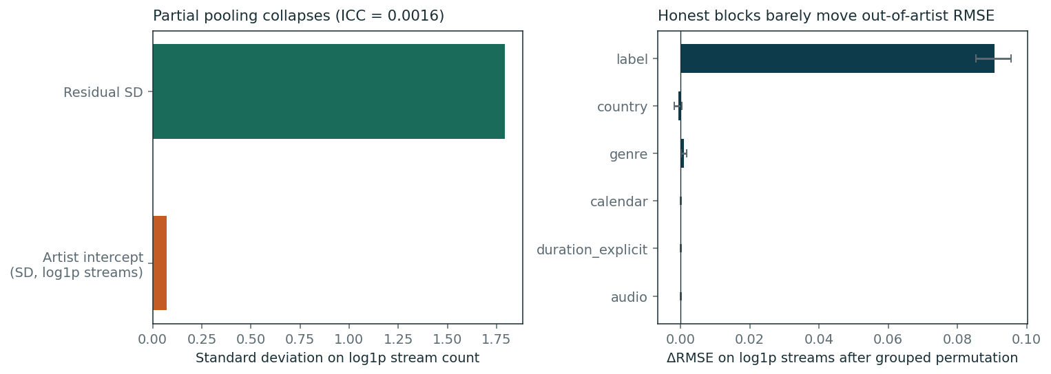
ALE on energy, loudness, danceability and tempo is visually flat relative to residual scale (the functions live in artifacts/uncertainty.json). Grouped permutation of the audio block moves held-out RMSE by essentially zero. The only block with a detectable δRMSE is label — a 30-level factor that can absorb a little mean shift, not a story about sound.

5. The planted tail is catalog size

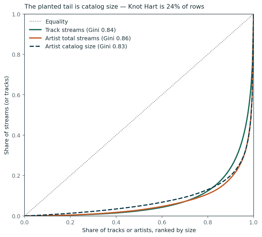
Streaming is a superstar economy in the row counts, not in quality per track. Mean streams per track are uncorrelated with how many rows an artist received ((r \approx 0)). Total streams are catalog size ((r = 0.995)).

pl = dist["track_streams"]["powerlaw"]
print("Track-stream CSN: xmin = {:.0f}, α = {:.3f}, n_tail = {:,}, KS = {:.3f}".format(
    pl["xmin"], pl["alpha"], pl["n_tail"], pl["ks"]))
print("GOF bootstrap p = {:.3f} (n_boot = {})".format(pl["gof"]["p_value"], pl["gof"]["n_boot"]))
print("Vuong PL vs lognormal: z = {:.1f}, p = {:.3g}".format(
    pl["vuong_pl_vs_lognormal"]["z"], pl["vuong_pl_vs_lognormal"]["p_value"]))
print("Vuong PL vs stretched exponential: z = {:.1f}, p = {:.3g}".format(
    pl["vuong_pl_vs_stretched_exp"]["z"], pl["vuong_pl_vs_stretched_exp"]["p_value"]))
g = dist["track_streams"]["gini"]
print("Track Gini = {:.3f} (95% bootstrap CI {:.3f}–{:.3f})".format(g["gini"], g["ci95"][0], g["ci95"][1]))
print(dist["survivorship"])

Track-stream CSN: xmin = 85770, α = 1.861, n_tail = 10,001, KS = 0.056
GOF bootstrap p = 0.012 (n_boot = 80)
Vuong PL vs lognormal: z = 29.1, p = 1.19e-186
Vuong PL vs stretched exponential: z = 41.3, p = 0
Track Gini = 0.837 (95% bootstrap CI 0.831–0.842)
500 named artists is a truncated sample whose mass sits in a planted tail: one invented artist is 24% of rows. Every tail index and Gini here describes that generator, not Spotify.

Clauset–Shalizi–Newman on track streams: (x_{\min}) chosen by KS on a geometric grid, α by MLE, GOF from the semi-parametric bootstrap. The power-law GOF rejects ((p = 0.012); none of 80 synthetic draws were more extreme than the observed KS). Relative to lognormal and stretched exponential on the same tail, Vuong still prefers the Pareto. That combination is the honest report: a truncated tail can look more Pareto than lognormal and still fail an absolute GOF test. It is also a property of the script that planted a heavy tail, not of Spotify.

Year-by-year Gini barely moves. The years were drawn as exchangeable.

Survivorship. Five hundred named artists whose mass sits in one invented catalog (Knot Hart, 24% of rows) is truncation by design. Every tail index above describes that generator.

6. Intervals that cover

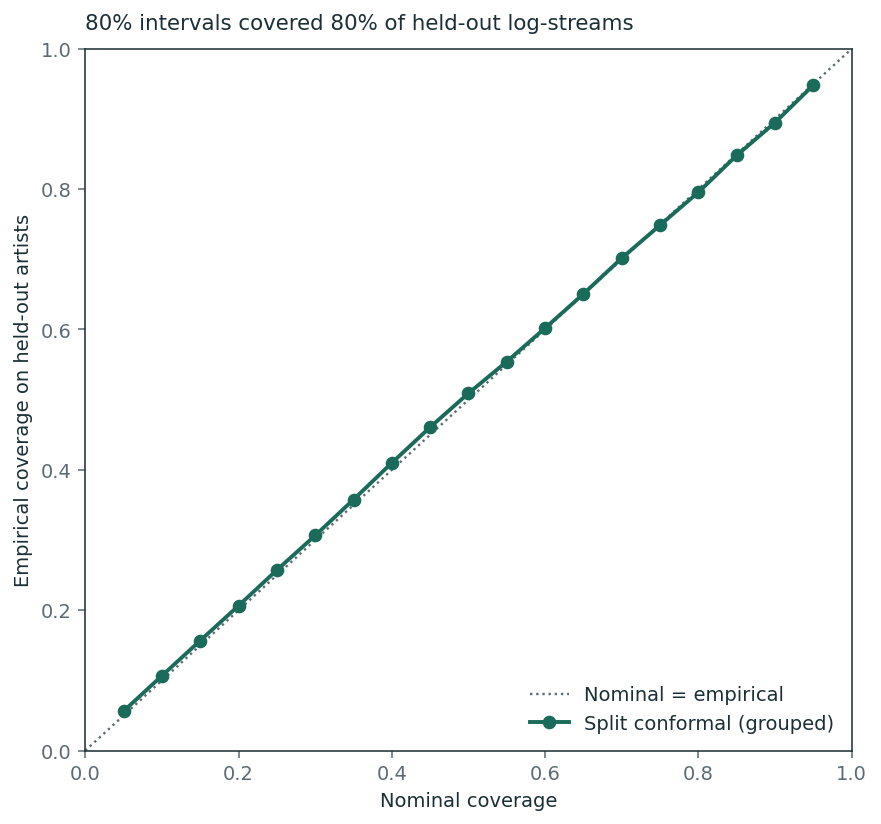
Split conformal residuals, with artists held out of fit, calibration and test. Nominal 80% intervals covered 80% of held-out log-streams. The curve sits on the diagonal because the honest model is close to a constant plus noise; conformal does not need a good mean function to be calibrated, and that is the point of reporting it.

cov = pd.DataFrame(unc["conformal"]["coverage"]).T
display(cov[["nominal", "empirical", "median_width"]].astype(float).round(3))
print("Test artists:", unc["conformal"]["n_test_artists"])

	nominal	empirical	median_width
0.5	0.5	0.509	2.451
0.8	0.8	0.796	4.562
0.9	0.9	0.895	5.726

Test artists: 125

7. What I would do with real data

• Listening events, not a release calendar. ListenBrainz gives actual plays. MusicBrainz gives canonical artist identity. That is a panel. This file is not.

• Weekly charts, not invented catalogs. Pre-API-sunset Spotify Chart dumps (or kworb archives) support seasonal adjustment, a 2020 level-shift with partial recovery, and hierarchical reconciliation of country × genre totals. That is where X-13ARIMA-SEATS and MinT belong. They do not belong on a synthetic calendar with a point mass on every day of 2020–2025.

• Audio features from a dump. Spotify closed the audio-features endpoint to new apps in November 2024. AcousticBrainz / Essentia, or an existing licensed dump, is the legal route. I would not scrape.

• A sampling frame. 500 known names are the tail. Estimating a power-law exponent from the tail you can see, without a model for truncation, is how those exponents get over-interpreted.

Phase 5 of the original brief — artist-level decomposition, COVID intervention regressors, MinT — is dropped here because the grain cannot support it. That is the methodological judgement, not a missing plot.

Audio features were unused for streams. They are not unused for planted genre: Genre from audio →.

Reproducibility

• Seed 20260903.

• make all in projects/spotify-power-laws runs 00_download.py … 09_genre.py.

• CSV is not committed; SHA-256 is in artifacts/download.json.

• Package: src/spotify_powerlaws/. Notebooks do not fit models.