library(tidyterra)
library(terra)
library(geodata)
library(rnaturalearth)
library(ggplot2)
library(dplyr)
library(sf)
library(rlang)
library(knitr)
library(patchwork)
library(leaflet)
library(htmlwidgets)
library(htmltools)
library(raster)
library(IRdisplay)
Attaching package: ‘tidyterra’
The following object is masked from ‘package:stats’:

    filter
terra 1.9.46
Attaching package: ‘dplyr’
The following objects are masked from ‘package:terra’:

    intersect, union
The following objects are masked from ‘package:stats’:

    filter, lag
The following objects are masked from ‘package:base’:

    intersect, setdiff, setequal, union
Linking to GEOS 3.12.1, GDAL 3.8.4, PROJ 9.4.0; sf_use_s2() is TRUE
Attaching package: ‘knitr’
The following object is masked from ‘package:terra’:

    spin
Attaching package: ‘patchwork’
The following object is masked from ‘package:terra’:

    area
Loading required package: sp
Attaching package: ‘raster’
The following object is masked from ‘package:dplyr’:

    select
The following object is masked from ‘package:tidyterra’:

    select
United Rugby Championship (URC)#
The United Rugby Championship spans Ireland, the United Kingdom (including Northern Ireland), Wales, Scotland, Italy, and South Africa. Unlike the English Premiership notebook, we cannot use a single GBR elevation tile: we pull SRTM 30 arc-second rasters from geodata::elevation_30s() for IRL, GBR, ITA, and ZAF, then sample the correct national raster for each stadium so we never merge full-country grids in memory.
Stadium coordinates below are approximate centre points for each club’s usual home ground (sources: club / venue pages and maps). If you need survey-grade coordinates or a different season’s venues, replace the urc_clubs table and rebuild.
urc_clubs <- data.frame(
  club = c(
    "Leinster", "Munster", "Ulster", "Connacht",
    "Glasgow Warriors", "Edinburgh",
    "Cardiff Rugby", "Ospreys", "Scarlets", "Dragons",
    "Benetton", "Zebre Parma",
    "Bulls", "Stormers", "Sharks", "Lions"
  ),
  stadium = c(
    "RDS Arena", "Thomond Park", "Kingspan Stadium", "The Sportsground",
    "Scotstoun Stadium", "Scottish Gas Murrayfield",
    "Cardiff Arms Park", "Swansea.com Stadium", "Parc y Scarlets", "Rodney Parade",
    "Stadio Monigo", "Stadio Lanfranchi",
    "Loftus Versfeld", "DHL Stadium", "Hollywoodbets Kings Park", "Emirates Airline Park"
  ),
  lon = c(
    -6.226, -8.618, -5.943, -9.077,
    -4.335, -3.240,
    -3.170, -3.941, -4.128, -2.991,
    12.229, 10.333,
    28.229, 18.411, 31.030, 28.061
  ),
  lat = c(
    53.325, 52.674, 54.576, 53.279,
    55.881, 55.942,
    51.479, 51.693, 51.679, 51.588,
    45.683, 44.800,
    -25.748, -33.903, -29.825, -26.198
  ),
  country = c(
    "Ireland", "Ireland", "United Kingdom", "Ireland",
    "United Kingdom", "United Kingdom",
    "United Kingdom", "United Kingdom", "United Kingdom", "United Kingdom",
    "Italy", "Italy",
    "South Africa", "South Africa", "South Africa", "South Africa"
  ),
  elev_source = c(
    "IRL", "IRL", "GBR", "IRL",
    "GBR", "GBR",
    "GBR", "GBR", "GBR", "GBR",
    "ITA", "ITA",
    "ZAF", "ZAF", "ZAF", "ZAF"
  ),
  stringsAsFactors = FALSE
)

urc_sv <- terra::vect(urc_clubs, geom = c("lon", "lat"), crs = "EPSG:4326")
Download elevation tiles (once per country)#
td <- tempdir()
elev_tiles <- list(
  IRL = geodata::elevation_30s(country = "IRL", path = td),
  GBR = geodata::elevation_30s(country = "GBR", path = td),
  ITA = geodata::elevation_30s(country = "ITA", path = td),
  ZAF = geodata::elevation_30s(country = "ZAF", path = td)
)

for (nm in names(elev_tiles)) {
  names(elev_tiles[[nm]]) <- paste0("elev_", nm)
}
Cached as: /tmp/RtmpfJDbBN/elevation/IRL_elv_msk.zip
Cached as: /tmp/RtmpfJDbBN/elevation/GBR_elv_msk.zip
Cached as: /tmp/RtmpfJDbBN/elevation/ITA_elv_msk.zip
Cached as: /tmp/RtmpfJDbBN/elevation/ZAF_elv_msk.zip
Extract elevation per ground#
extract_point_elev <- function(lon, lat, src) {
  r <- elev_tiles[[src]]
  pts <- terra::vect(
    data.frame(lon = lon, lat = lat),
    geom = c("lon", "lat"),
    crs = "EPSG:4326"
  )
  if (!terra::same.crs(r, pts)) {
    pts <- terra::project(pts, r)
  }
  ex <- terra::extract(r, pts)
  as.numeric(ex[[names(r)[1]]])
}

urc_elev <- urc_clubs |>
  mutate(
    ground_elevation_m = mapply(
      extract_point_elev,
      lon,
      lat,
      elev_source,
      USE.NAMES = FALSE
    )
  )

urc_elev |>
  arrange(desc(ground_elevation_m)) |>
  knitr::kable(
    digits = 1,
    caption = "URC grounds ranked by extracted elevation (m a.s.l.; national SRTM tile)"
  )
Table: URC grounds ranked by extracted elevation (m a.s.l.; national SRTM tile)

|club             |stadium                  |  lon|   lat|country        |elev_source | ground_elevation_m|
|:----------------|:------------------------|----:|-----:|:--------------|:-----------|------------------:|
|Lions            |Emirates Airline Park    | 28.1| -26.2|South Africa   |ZAF         |               1727|
|Bulls            |Loftus Versfeld          | 28.2| -25.7|South Africa   |ZAF         |               1385|
|Ospreys          |Swansea.com Stadium      | -3.9|  51.7|United Kingdom |GBR         |                107|
|Zebre Parma      |Stadio Lanfranchi        | 10.3|  44.8|Italy          |ITA         |                 66|
|Edinburgh        |Scottish Gas Murrayfield | -3.2|  55.9|United Kingdom |GBR         |                 47|
|Ulster           |Kingspan Stadium         | -5.9|  54.6|United Kingdom |GBR         |                 26|
|Connacht         |The Sportsground         | -9.1|  53.3|Ireland        |IRL         |                 16|
|Benetton         |Stadio Monigo            | 12.2|  45.7|Italy          |ITA         |                 16|
|Cardiff Rugby    |Cardiff Arms Park        | -3.2|  51.5|United Kingdom |GBR         |                 15|
|Stormers         |DHL Stadium              | 18.4| -33.9|South Africa   |ZAF         |                 15|
|Glasgow Warriors |Scotstoun Stadium        | -4.3|  55.9|United Kingdom |GBR         |                 12|
|Sharks           |Hollywoodbets Kings Park | 31.0| -29.8|South Africa   |ZAF         |                 10|
|Leinster         |RDS Arena                | -6.2|  53.3|Ireland        |IRL         |                  9|
|Scarlets         |Parc y Scarlets          | -4.1|  51.7|United Kingdom |GBR         |                  9|
|Dragons          |Rodney Parade            | -3.0|  51.6|United Kingdom |GBR         |                  9|
|Munster          |Thomond Park             | -8.6|  52.7|Ireland        |IRL         |                  4|
The bar chart orders clubs from lowest to highest extracted elevation using the same values as the table.
urc_bar <- urc_elev |>
  mutate(club = stats::reorder(club, ground_elevation_m))

ggplot(urc_bar, aes(x = club, y = ground_elevation_m, fill = country)) +
  geom_col(width = 0.78, colour = "grey35", linewidth = 0.25) +
  coord_flip() +
  scale_fill_brewer(palette = "Set3", name = "Country") +
  labs(
    title = "URC ground elevation (ascending)",
    x = NULL,
    y = "Elevation (m a.s.l.)"
  ) +
  theme_minimal(base_size = 11) +
  theme(
    plot.title = element_text(face = "bold", hjust = 0, margin = margin(b = 8)),
    panel.grid.major.y = element_blank(),
    panel.grid.minor = element_blank(),
    legend.position = "bottom"
  )
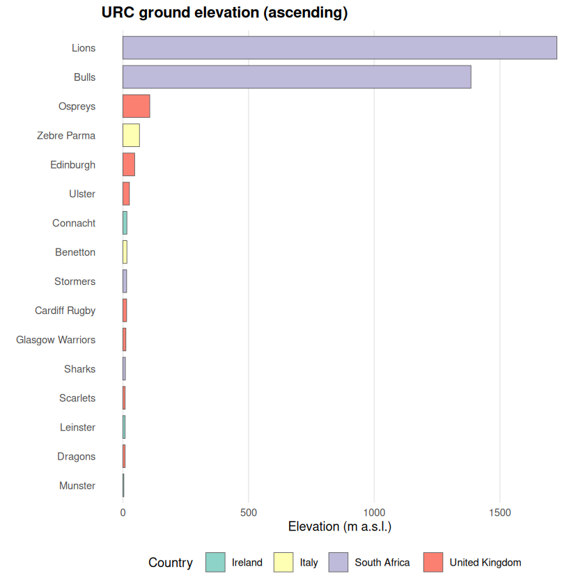
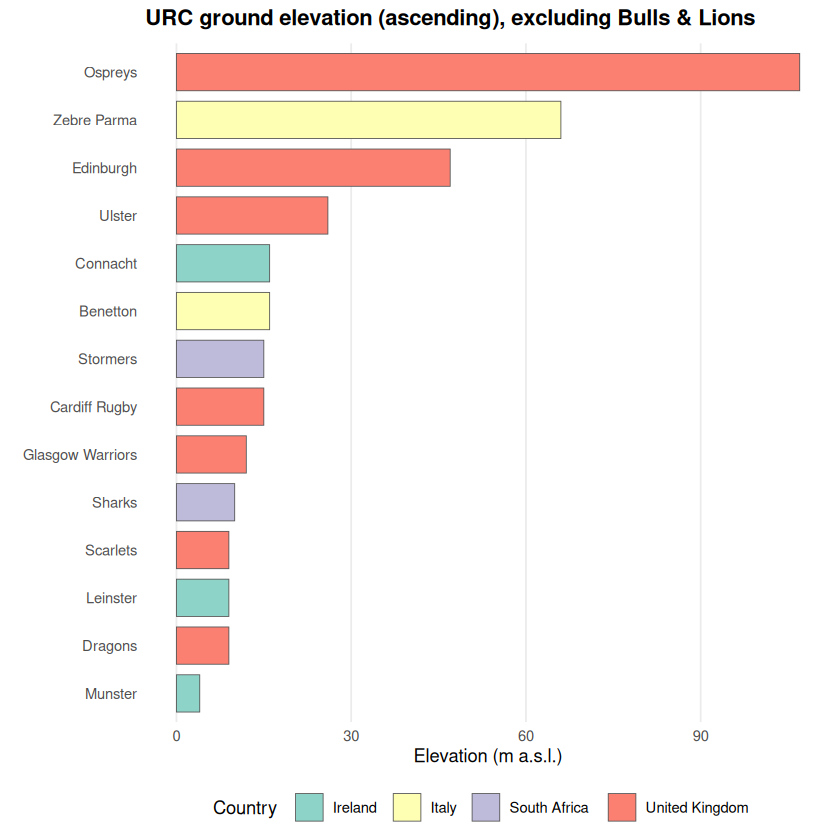
Bulls and Lions both play on the South African Highveld (Johannesburg and Pretoria), where the 30 arc-second DEM routinely returns roughly 1.2–1.7 km above sea level. Those two values sit far above every European and coastal URC ground, so the first chart’s vertical scale is dominated by them: differences of a few tens of metres between, say, Irish and Welsh venues are visually squashed.
Dropping Bulls and Lions for a second view is therefore a deliberate outlier removal for readability—not a claim they are “wrong”, but a way to stretch the axis so relative ordering among the remaining fourteen clubs is visible.
urc_bar_trim <- urc_elev |>
  dplyr::filter(!club %in% c("Bulls", "Lions")) |>
  mutate(club = stats::reorder(club, ground_elevation_m))

ggplot(urc_bar_trim, aes(x = club, y = ground_elevation_m, fill = country)) +
  geom_col(width = 0.78, colour = "grey35", linewidth = 0.25) +
  coord_flip() +
  scale_fill_brewer(palette = "Set3", name = "Country") +
  labs(
    title = "URC ground elevation (ascending), excluding Bulls & Lions",
    x = NULL,
    y = "Elevation (m a.s.l.)"
  ) +
  theme_minimal(base_size = 11) +
  theme(
    plot.title = element_text(face = "bold", hjust = 0, margin = margin(b = 8)),
    panel.grid.major.y = element_blank(),
    panel.grid.minor = element_blank(),
    legend.position = "bottom"
  )
Regional maps (Europe and South Africa)#
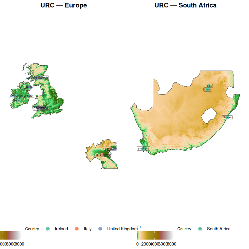
European URC clubs sit on IRL / GBR / ITA tiles; South African sides use ZAF. We crop each national raster to a modest bounding box around the relevant grounds, merge the European crops for one hypsometric panel, and show South Africa separately so the aspect scales remain readable.
world_sf <- rnaturalearth::ne_countries(scale = "medium", returnclass = "sf")
urc_outline_sf <- world_sf[world_sf$iso_a3 %in% c("GBR", "IRL", "ITA", "ZAF"), ]
urc_outline <- terra::vect(urc_outline_sf)

eur_df <- urc_clubs |> dplyr::filter(elev_source != "ZAF")
sa_df <- urc_clubs |> dplyr::filter(elev_source == "ZAF")

eur_ext <- terra::extend(terra::ext(terra::vect(eur_df, geom = c("lon", "lat"), crs = "EPSG:4326")), 2)
sa_ext <- terra::extend(terra::ext(terra::vect(sa_df, geom = c("lon", "lat"), crs = "EPSG:4326")), 2)

r_eur <- terra::merge(
  terra::crop(elev_tiles$IRL, eur_ext),
  terra::merge(
    terra::crop(elev_tiles$GBR, eur_ext),
    terra::crop(elev_tiles$ITA, eur_ext)
  )
)
names(r_eur) <- "elevation"

r_sa <- terra::crop(elev_tiles$ZAF, sa_ext)
names(r_sa) <- "elevation"

eur_pts <- terra::vect(eur_df, geom = c("lon", "lat"), crs = "EPSG:4326")
sa_pts <- terra::vect(sa_df, geom = c("lon", "lat"), crs = "EPSG:4326")

outline_eur <- terra::crop(urc_outline, eur_ext)
outline_sa <- terra::crop(urc_outline, sa_ext)

if (!terra::same.crs(r_eur, outline_eur)) {
  outline_eur <- terra::project(outline_eur, r_eur)
}
if (!terra::same.crs(r_sa, outline_sa)) {
  outline_sa <- terra::project(outline_sa, r_sa)
}
p_eur <- ggplot() +
  tidyterra::geom_spatraster(data = r_eur, aes(fill = elevation)) +
  tidyterra::scale_fill_hypso_tint_c(
    name = "m",
    guide = guide_colorbar(barwidth = unit(2.6, "cm"), title.position = "top")
  ) +
  tidyterra::geom_spatvector(data = eur_pts, aes(colour = country), size = 2.8, show.legend = TRUE) +
  tidyterra::geom_spatvector_label(
    data = eur_pts,
    aes(label = club),
    size = 2,
    colour = "grey10",
    label.size = 0.12,
    show.legend = FALSE
  ) +
  tidyterra::geom_spatvector(data = outline_eur, fill = NA, colour = "grey25", linewidth = 0.25) +
  scale_colour_brewer(palette = "Set2", name = "Country") +
  labs(title = "URC — Europe") +
  theme_void() +
  theme(
    plot.title = element_text(face = "bold", hjust = 0.5, margin = margin(b = 4)),
    legend.title = element_text(size = 8),
    legend.position = "bottom"
  )

p_sa <- ggplot() +
  tidyterra::geom_spatraster(data = r_sa, aes(fill = elevation)) +
  tidyterra::scale_fill_hypso_tint_c(
    name = "m",
    guide = guide_colorbar(barwidth = unit(2.6, "cm"), title.position = "top")
  ) +
  tidyterra::geom_spatvector(data = sa_pts, aes(colour = country), size = 2.8, show.legend = TRUE) +
  tidyterra::geom_spatvector_label(
    data = sa_pts,
    aes(label = club),
    size = 2,
    colour = "grey10",
    label.size = 0.12,
    show.legend = FALSE
  ) +
  tidyterra::geom_spatvector(data = outline_sa, fill = NA, colour = "grey25", linewidth = 0.25) +
  scale_colour_brewer(palette = "Set2", name = "Country") +
  labs(title = "URC — South Africa") +
  theme_void() +
  theme(
    plot.title = element_text(face = "bold", hjust = 0.5, margin = margin(b = 4)),
    legend.title = element_text(size = 8),
    legend.position = "bottom"
  )

p_eur + p_sa + patchwork::plot_layout(ncol = 2, widths = c(1, 1))
<SpatRaster> resampled to 501410 cells.
Warning message:
“The `label.size` argument of `geom_label()` is deprecated as of ggplot2 3.5.0.
ℹ Please use the `linewidth` argument instead.
ℹ The deprecated feature was likely used in the tidyterra package.
  Please report the issue at <https://github.com/dieghernan/tidyterra/issues>.”
<SpatRaster> resampled to 500286 cells.
Warning message in st_point_on_surface.sfc(sf::st_zm(x)):
“st_point_on_surface may not give correct results for longitude/latitude data”
Warning message in st_point_on_surface.sfc(sf::st_zm(x)):
“st_point_on_surface may not give correct results for longitude/latitude data”
Interactive maps#
The maps below use Leaflet (via htmlwidgets). You can pan, zoom, and click stadium markers for club, venue, and extracted elevation. Marker colours follow the same elevation colour scale as the terrain layer. An internet connection is required for the light basemap tiles.
URC — Europe (interactive)
URC — South Africa (interactive)
Coastal Stormers and Sharks grounds are often only a few metres above sea level in the DEM, while Bulls and Lions sit on the Highveld at roughly 1.3–1.7 km—patterns that read clearly in both the bar chart and the South Africa panel.