Fay–Herriot: Bayesian hierarchical model#
Navigation: ← Previous: Classical EBLUP | Next: Model Comparison →
The same area-level model, now with a joint posterior over \((\theta, \beta, \sigma_u^2)\). A conjugate Gibbs sampler is the workhorse; a PyMC NUTS fit is the independent check.
import sys
from pathlib import Path
import pandas as pd
import numpy as np
import matplotlib.pyplot as plt
import plotly.graph_objects as go
import plotly.express as px
from IPython.display import HTML, display
import warnings
warnings.filterwarnings('ignore')
plt.style.use('seaborn-v0_8-whitegrid')

PROJ_DIR = Path('.').resolve()
if not (PROJ_DIR / 'sae_utils.py').exists():
    PROJ_DIR = Path('projects/small-area-estimation').resolve()
if str(PROJ_DIR) not in sys.path:
    sys.path.insert(0, str(PROJ_DIR))

from sae_utils import (
    load_panel, modelling_frame, design_matrix, eblup_fh, fh_reml_sigma_u,
    jackknife_mse, gibbs_fh, summarise_theta, posterior_predictive_y,
    rhat_split, coverage_rate, project_data_dir,
)

def display_plotly(fig):
    """Embed Plotly with CDN JS — fig.show() is blank in Jupyter Book HTML."""
    display(HTML(fig.to_html(include_plotlyjs='cdn', full_html=False)))

FIG_DIR = PROJ_DIR / 'figures'
FIG_DIR.mkdir(exist_ok=True)
DATA_DIR = project_data_dir()
PANEL = load_panel()
MODEL = modelling_frame(PANEL)
print(f'Panel: {len(PANEL)} local authorities; modelling subset: {len(MODEL)}')
print(f'Period (APS / ONS model-based): {PANEL["direct_period"].dropna().iloc[0]}')
Panel: 348 local authorities; modelling subset: 136
Period (APS / ONS model-based): Apr 2025-Mar 2026
Why Bayes here#
The EBLUP is a posterior mean for \(\theta_i\) under a flat prior on \(\beta\) and a plug-in \(\hat\sigma_u^2\). That plug-in step is the awkward bit: \(g_3\) is a Taylor correction for not knowing \(\sigma_u^2\). A hierarchical Bayesian model just samples it.
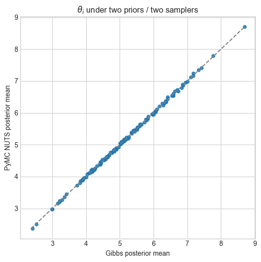
This is conjugate, so Gibbs is exact (up to Monte Carlo) and cheap. NUTS in PyMC does not need conjugacy; we use it to confirm that the posterior is not an artefact of the Inverse-Gamma prior. A half-normal on \(\sigma_u\) (PyMC) and IG\((0.5,0.5)\) on \(\sigma_u^2\) (Gibbs) are not the same prior — if \(\theta_i\) posteriors still agree, the likelihood is doing the work.
That last point is the frequentist/Bayes distinction that actually matters here. It is not that one produces point estimates and the other intervals. Both produce both. The difference is whether uncertainty in \(\sigma_u^2\) is a correction term or a sampled parameter, and whether you are willing to insert a prior that remains informative when \(m\) is small.
Gibbs sampler#
Full conditionals (Gelman et al. notation; scale parameterisation of IG):
\(\theta_i \mid \cdot \sim N\big(v_i(y_i/\psi_i + x_i'\beta/\sigma_u^2),\, v_i\big)\), \(v_i^{-1} = \psi_i^{-1} + \sigma_u^{-2}\)
\(\beta \mid \cdot \sim N(m_\beta, V_\beta)\) with precision \(X'X/\sigma_u^2 + \tau^{-2}I\)
\(\sigma_u^2 \mid \cdot \sim \mathrm{IG}(a+m/2,\, b + \tfrac12\|\theta-X\beta\|^2)\)
\(\tau^2 = 10^4\) is weakly informative on the percentage-point scale.
gibbs = gibbs_fh(MODEL, covariates=['claimant_rate'], draws=4000, burn=1000, thin=2, seed=42)
theta_g = gibbs['theta']
sum_g = summarise_theta(theta_g, index=MODEL.index)
bayes = MODEL.join(sum_g)
print(f"Kept draws: {gibbs['draws']}")
print(f"Posterior mean σ²_u = {gibbs['sigma_u2'].mean():.3f}  "
      f"median={np.median(gibbs['sigma_u2']):.3f}")
print('β posterior means:', dict(zip(gibbs['coef_names'], np.round(gibbs['beta'].mean(0), 3))))
for i, name in enumerate(gibbs['coef_names']):
    d = gibbs['beta'][:, i]
    print(f"  {name}: mean={d.mean():.3f}  95% CI=({np.quantile(d,0.025):.3f}, {np.quantile(d,0.975):.3f})")
print(f"split-R̂(σ²_u) ≈ {rhat_split(gibbs['sigma_u2']):.3f}")
bayes[['GEOGRAPHY_NAME','direct_rate','bayes_mean','bayes_ci_lo','bayes_ci_hi']].head()
Kept draws: 1500
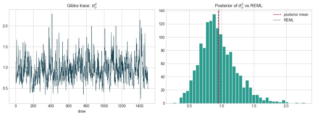
Posterior mean σ²_u = 0.949  median=0.908
β posterior means: {'intercept': np.float64(2.38), 'claimant_rate': np.float64(0.651)}
  intercept: mean=2.380  95% CI=(1.598, 3.181)
  claimant_rate: mean=0.651  95% CI=(0.472, 0.835)
split-R̂(σ²_u) ≈ 1.004
| GEOGRAPHY_NAME | direct_rate | bayes_mean | bayes_ci_lo | bayes_ci_hi | |
|---|---|---|---|---|---|
| 0 | Barking and Dagenham | 6.1 | 6.951729 | 5.193146 | 8.662916 |
| 1 | Barnet | 5.5 | 5.587427 | 4.068580 | 7.265468 |
| 2 | Barnsley | 2.6 | 3.356316 | 2.140859 | 4.516208 |
| 3 | Bath and North East Somerset | 4.6 | 4.038717 | 2.719589 | 5.446427 |
| 4 | Bexley | 7.3 | 5.172318 | 3.536707 | 6.882331 |
fig, axes = plt.subplots(1, 2, figsize=(12, 4.5))
axes[0].plot(gibbs['sigma_u2'], lw=0.6, color='#0d3b4c')
axes[0].set_title(r'Gibbs trace: $\sigma_u^2$')
axes[0].set_xlabel('draw')
axes[1].hist(gibbs['sigma_u2'], bins=40, color='#2a9d8f', edgecolor='white')
axes[1].axvline(gibbs['sigma_u2'].mean(), color='crimson', ls='--', label='posterior mean')
e = eblup_fh(MODEL, covariates=['claimant_rate'])
axes[1].axvline(e.attrs['fit']['sigma_u2'], color='black', ls=':', label='REML')
axes[1].set_title(r'Posterior of $\sigma_u^2$ vs REML')
axes[1].legend()
fig.tight_layout()
fig.savefig(FIG_DIR / '05_sigma_u_posterior.png', dpi=120)
fig
PyMC / NUTS#
The non-conjugate specification puts a half-normal prior on \(\sigma_u\) and independent \(N(0,10^2)\) priors on \(\beta\). If PyMC is unavailable in this runtime, the cell records the failure and the Gibbs posterior remains the Bayesian result.
pymc_ok = False
pymc_sum = None
try:
    from sae_utils import fit_pymc_fh
    pymc_fit = fit_pymc_fh(
        MODEL, covariates=['claimant_rate'],
        draws=600, tune=600, chains=2, seed=42,
    )
    pymc_sum = summarise_theta(pymc_fit['theta'], index=MODEL.index).add_prefix('pymc_')
    pymc_ok = True
    print(f"NUTS draws: {pymc_fit['draws']}")
    print(f"Posterior mean σ²_u (NUTS) = {pymc_fit['sigma_u2'].mean():.3f}")
    print(f"split-R̂(σ_u) ≈ {rhat_split(np.sqrt(pymc_fit['sigma_u2'])):.3f}")
except Exception as exc:
    print('PyMC fit skipped:', type(exc).__name__, '-', exc)
Initializing NUTS using jitter+adapt_diag...
Sequential sampling (2 chains in 1 job)
NUTS: [sigma_u, beta, theta]
Sampling 2 chains for 600 tune and 600 draw iterations (1_200 + 1_200 draws total) took 1 seconds.
There was 1 divergence after tuning. Increase `target_accept` or reparameterize.
We recommend running at least 4 chains for robust computation of convergence diagnostics
The rhat statistic is larger than 1.01 for some parameters. This indicates problems during sampling. See https://arxiv.org/abs/1903.08008 for details
NUTS draws: 1200
Posterior mean σ²_u (NUTS) = 0.973
split-R̂(σ_u) ≈ 1.002
if pymc_ok:
    cmp = pd.DataFrame({
        'gibbs_mean': bayes['bayes_mean'],
        'pymc_mean': pymc_sum['pymc_bayes_mean'],
    })
    print('corr(Gibbs, NUTS) θ means:', np.corrcoef(cmp['gibbs_mean'], cmp['pymc_mean'])[0,1].round(4))
    print((cmp['gibbs_mean'] - cmp['pymc_mean']).describe().round(3))
    fig, ax = plt.subplots(figsize=(5.5, 5.5))
    ax.scatter(cmp['gibbs_mean'], cmp['pymc_mean'], s=22, alpha=0.85)
    lims = [cmp.min().min(), cmp.max().max()]
    ax.plot(lims, lims, '--', color='grey')
    ax.set_xlabel('Gibbs posterior mean')
    ax.set_ylabel('PyMC NUTS posterior mean')
    ax.set_title(r'$\theta_i$ under two priors / two samplers')
    fig.tight_layout()
    fig.savefig(FIG_DIR / '05_gibbs_vs_pymc.png', dpi=120)
    fig
else:
    print('No NUTS comparison in this runtime.')
corr(Gibbs, NUTS) θ means: 0.9998
count    136.000
mean      -0.001
std        0.026
min       -0.079
25%       -0.019
50%        0.001
75%        0.017
max        0.059
dtype: float64
Posterior predictive check#
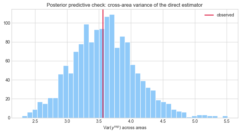
Draw \(y_i^{\mathrm{rep}} \sim N(\theta_i^{(s)}, \psi_i)\) and compare the replicated distribution of, say, the cross-area variance of \(y\) to the observed one. A linking model that is too rigid (tiny \(\sigma_u^2\)) under-replicates the spread of the direct estimates; one that ignores \(\psi_i\) over-replicates it.
y = MODEL['direct_rate'].to_numpy()
psi = MODEL['psi'].to_numpy()
y_rep = posterior_predictive_y(theta_g, psi, seed=1)
obs_var = y.var(ddof=1)
rep_var = y_rep.var(axis=1, ddof=1)
pval = (rep_var >= obs_var).mean()
print(f'Observed Var(y) = {obs_var:.3f}')
print(f'Replicated mean Var(y) = {rep_var.mean():.3f}  (PPP = {pval:.3f})')
fig, ax = plt.subplots(figsize=(8, 4.5))
ax.hist(rep_var, bins=40, color='#90caf9', edgecolor='white')
ax.axvline(obs_var, color='crimson', lw=2, label='observed')
ax.set_xlabel(r'Var$(y^{rep})$ across areas')
ax.set_title('Posterior predictive check: cross-area variance of the direct estimator')
ax.legend()
fig.tight_layout()
fig.savefig(FIG_DIR / '05_ppc_variance.png', dpi=120)
fig
Observed Var(y) = 3.562
Replicated mean Var(y) = 3.587  (PPP = 0.515)
Key takeaways#
The Bayesian \(\theta_i\) posterior mean is an EBLUP with \(\sigma_u^2\) integrated rather than plugged in; it should sit close to the REML EBLUP when \(m\) is large.
Credible intervals automatically include uncertainty in \(\beta\) and \(\sigma_u^2\). They still assume \(\psi_i\) known and \(u_i\) iid normal.
Prior disagreement (IG vs half-normal) is a feature: if Gibbs and NUTS diverge, the variance component is weakly identified and the EBLUP MSE formula is in the same fragile regime.
Navigation: ← Previous: Classical EBLUP | Next: Model Comparison →