Genre from audio

Navigation: ← Streams and leakage · Project overview

The generator coupled sound to genre, not to success.

Page 1 showed that audio features are orthogonal to streams. The publisher also claimed genre-specific audio distributions. That is a different estimand, and it is the unused signal. This page asks whether those features recover the planted genre label for a held-out artist.

Fitting lives in src/spotify_powerlaws/genre.py and scripts/09_genre.py. This notebook loads artifacts/genre.json.

import json
from pathlib import Path
import pandas as pd
from IPython.display import display

PROJ = Path(".").resolve()
if not (PROJ / "artifacts" / "genre.json").exists():
    PROJ = Path("projects/spotify-power-laws").resolve()

genre = json.loads((PROJ / "artifacts" / "genre.json").read_text())
print(genre["estimand"]["question"])
print("Classes:", genre["estimand"]["n_classes"])
print("Majority:", genre["majority_label"], f"{genre['majority_share']:.1%}")
print("Features:", ", ".join(genre["estimand"]["features"]))

Among tracks in this synthetic catalog, how well do antecedent audio features predict the planted genre label, with artist as the unit of independence?
Classes: 20
Majority: R&B 26.5%
Features: danceability, energy, loudness, instrumentalness, tempo, key, mode, duration_ms, explicit

Estimand

Target. genre, 20 nominal labels, track grain.

Question. Among tracks in this catalog, how well do antecedent audio features predict the planted genre, with artist as the unit of independence?

Features. danceability, energy, loudness, instrumentalness, tempo, key, mode, duration_ms, explicit. Not upbeat_score (a composite), not streams or popularity, not label or country.

Metrics. R&B is 26.5% of rows, so accuracy is a footnote. Lead with balanced accuracy, macro-F1, and log-loss. Chance balanced accuracy for 20 classes is (1/20 = 0.05).

Not identified. Real-world genre taxonomy, recommendation, Spotify listening, or stream prediction — page 1 already closed that.

Split. GroupKFold by artist_name. 460 of 500 artists span multiple genres, so this tests the audio–genre map, not “one genre per artist”. Shuffled k-fold is reported once as an optimism check.

The planted audio geometry

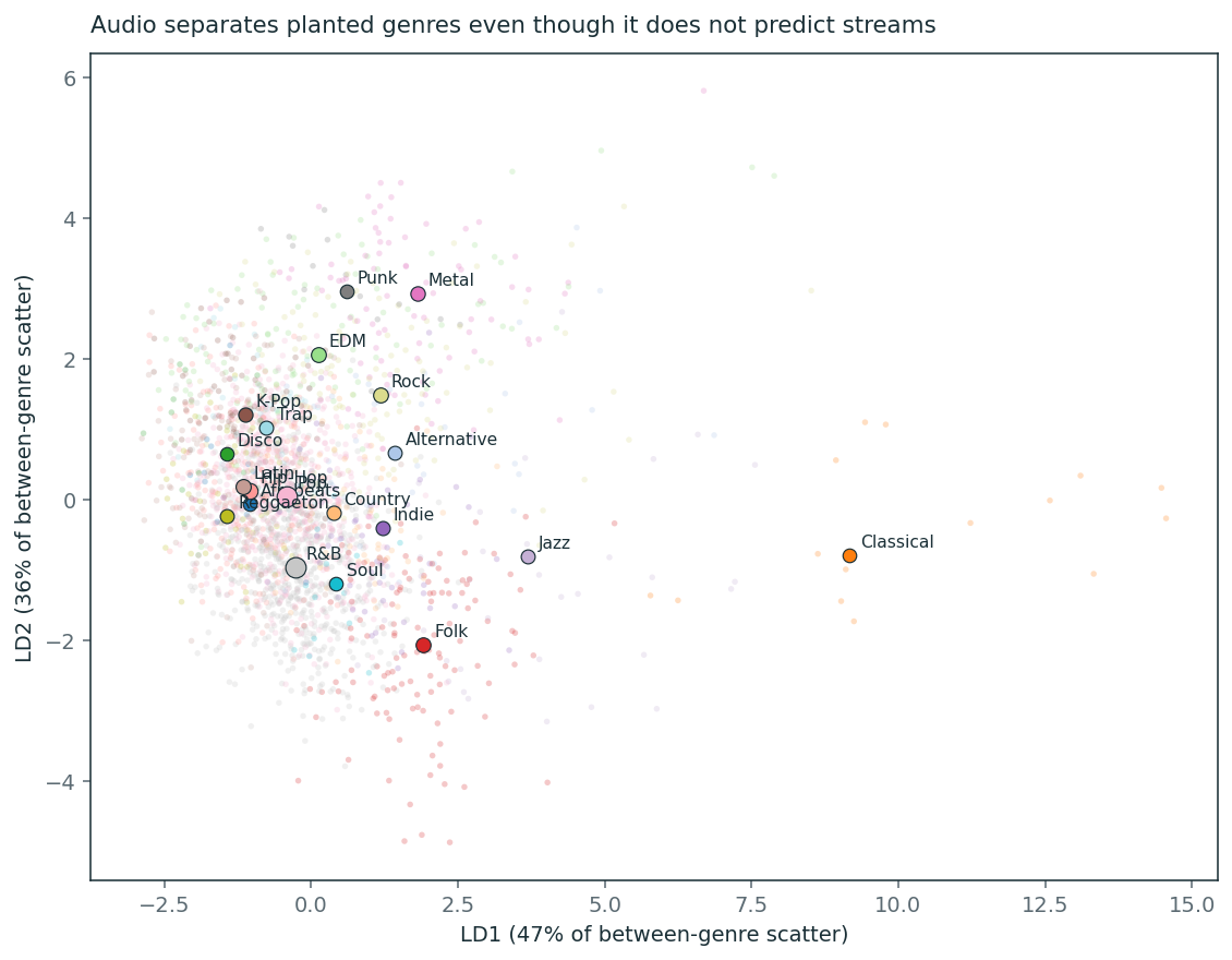
LDA is the natural model if the script drew genre-specific Gaussians. The first two discriminants are a descriptive view of that geometry, not a cross-validated score.

ev = genre["lda_coordinates"]["explained_variance_ratio"]
print(f"LD1+LD2 explain {sum(ev):.0%} of between-genre scatter ({ev[0]:.0%} + {ev[1]:.0%}).")
means = pd.DataFrame(genre["lda_coordinates"]["means"]).sort_values("n", ascending=False)
display(means.head(8).round(2))

LD1+LD2 explain 83% of between-genre scatter (47% + 36%).

	genre	ld1	ld2	n
15	R&B	-0.26	-0.95	13273
13	Pop	-0.41	0.04	12915
7	Hip-Hop	-1.05	0.13	3930
11	Latin	-1.17	0.19	2661
5	EDM	0.12	2.06	2407
17	Rock	1.18	1.49	2370
6	Folk	1.91	-2.06	2249
12	Metal	1.81	2.93	1695

Classical and jazz sit off to the side; metal and punk sit high on LD2; the pop-adjacent cluster (R&B, Pop, Hip-Hop, Latin, K-Pop, Trap) is a pile. That is what a 20-label generator with overlapping popular styles looks like. It is also why stream models could find energy–loudness structure and still have nothing to say about success.

Where the labels collide

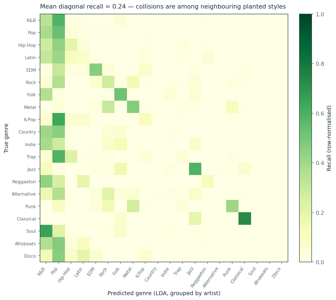
Grouped-CV predictions from LDA, row-normalised so rare classes are visible.

rare = pd.DataFrame(genre["per_class_lda_grouped"]["rarest_five"]).T
rare.columns = ["n", "recall"]
display(rare.round(3))
print("Mean diagonal recall (macro recall) = {:.3f}".format(
    sum(genre["per_class_lda_grouped"]["recall"].values()) / 20
))

	n	recall
Disco	198.0	0.000
Afrobeats	224.0	0.000
Soul	325.0	0.000
Classical	357.0	0.731
Punk	384.0	0.411

Mean diagonal recall (macro recall) = 0.245

Disco, Afrobeats and Soul have zero grouped-CV recall under LDA — they are absorbed into R&B and Pop. Classical is recovered at 0.73, punk at 0.41. Macro-F1 is a story about the tail of the label set, not about the two giant classes.

Ladder, then stop

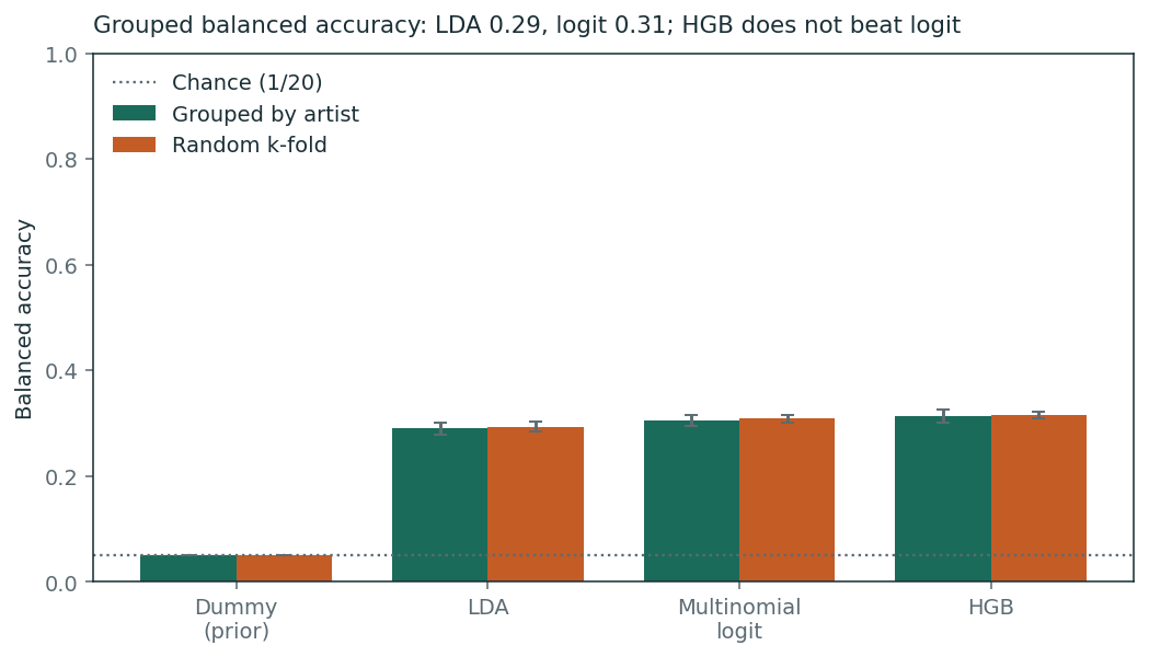
Dummy (class prior) → LDA → multinomial logit → histogram gradient boosting with early stopping. Same audio block. Outer-fold balanced accuracy, Nadeau–Bengio corrected (t) on the five grouped folds.

rows = []
for name, label in [
    ("dummy", "Dummy (prior)"),
    ("lda", "LDA"),
    ("logit", "Multinomial logit"),
    ("hgb", "HGB"),
]:
    g = genre["models"][f"{name}_grouped"]["summary"]
    r = genre["models"][f"{name}_random"]["summary"]
    rows.append({
        "model": label,
        "BA grouped": g["balanced_accuracy"]["mean"],
        "BA random": r["balanced_accuracy"]["mean"],
        "macro-F1 grouped": g["macro_f1"]["mean"],
        "log-loss grouped": g["log_loss"]["mean"],
        "accuracy grouped": g["accuracy"]["mean"],
        "accuracy random": r["accuracy"]["mean"],
    })
tab = pd.DataFrame(rows).set_index("model")
display(tab.round(3))
print("LDA random vs grouped BA relative lift: {:.1%}".format(genre["optimism_gap_lda_ba"]["relative_lift"]))
for name, test in genre["tests"].items():
    print(f"{name}: Δ = {test['mean_diff']:.4f}, t = {test['t']:.2f}, p = {test['p_value']:.3g}")

	BA grouped	BA random	macro-F1 grouped	log-loss grouped	accuracy grouped	accuracy random
model
Dummy (prior)	0.050	0.050	0.007	2.675	0.081	0.265
LDA	0.290	0.293	0.244	1.847	0.351	0.480
Multinomial logit	0.305	0.309	0.260	1.734	0.360	0.489
HGB	0.314	0.316	0.264	1.748	0.364	0.491

LDA random vs grouped BA relative lift: 1.0%
lda_vs_dummy_grouped: Δ = -0.2401, t = -30.08, p = 7.28e-06
logit_vs_lda_grouped: Δ = -0.0152, t = -4.56, p = 0.0104
hgb_vs_lda_grouped: Δ = -0.0238, t = -7.33, p = 0.00184
hgb_vs_logit_grouped: Δ = -0.0086, t = -2.22, p = 0.0903
lda_random_vs_grouped: Δ = -0.0030, t = -0.32, p = 0.764

Three results.

1. Audio does recover genre, modestly. LDA grouped balanced accuracy is 0.29 against a 0.05 dummy. The publisher’s “genre-specific audio” claim is visible in the file. It is not a strong classifier — and it does not need to be, to make the point.

2. Capacity stops at logit. Logit beats LDA by 1.5 points of balanced accuracy (corrected (t = -4.56), (p = 0.010)). HGB beats LDA but does not beat logit ((p = 0.090)). The extra trees are not a second model.

3. Random k-fold inflates accuracy, not balanced accuracy. LDA accuracy jumps from 0.35 grouped to 0.48 random, because one invented artist is 24% of rows and mostly R&B. Balanced accuracy barely moves (relative lift 1.0%, (p = 0.76)). Composition leakage shows up in the metric that rewards the modal class. That is the page 1 validation lesson, restated for a target the audio block can actually predict.

What this does not rehabilitate

Recovering planted genre from audio is a statement about the script that labelled tracks. It does not mean audio features drive listening, it does not make the stream-(R^2) of 0.05 look better, and it is not a recommendation model. The two pages together are the result: sound was coupled to genre; success was coupled to log_stream_count.

Reproducibility

• Seed 20260903.

• make genre runs scripts/09_genre.py.

• Artifact: artifacts/genre.json. Figures: 07_genre_lda.png, 08_genre_confusion.png, 09_genre_ladder.png.